
Special Issue Reprint
# EEG Signal Processing Techniques and Applications
Edited by Yifan Zhao, Fei He and Yuzhu Guo
mdpi.com/journal/sensors

# EEG Signal Processing Techniques and Applications
## EEG Signal Processing Techniques and Applications
Editors
**Yifan Zhao Fei He Yuzhu Guo**

Basel • Beijing • Wuhan • Barcelona • Belgrade • Novi Sad • Cluj • Manchester
*Editors*
Yifan Zhao
Cranfield University
Cranfield UK
Fei He
Coventry University
Coventry UK
Yuzhu Guo
Beihang University
Beijing China
*Editorial Office* MDPI St. Alban-Anlage 66 4052 Basel, Switzerland
This is a reprint of articles from the Special Issue published online in the open access journal *Sensors* (ISSN 1424-8220) (available at: https://www.mdpi.com/journal/sensors/special issues/ EEG Signal Processing Techniques).
For citation purposes, cite each article independently as indicated on the article page online and as indicated below:
Lastname, A.A.; Lastname, B.B. Article Title. *Journal Name* **Year**, *Volume Number*, Page Range.
**ISBN 978-3-7258-0081-0 (Hbk) ISBN 978-3-7258-0082-7 (PDF) doi.org/10.3390/books978-3-7258-0082-7**
© 2024 by the authors. Articles in this book are Open Access and distributed under the Creative Commons Attribution (CC BY) license. The book as a whole is distributed by MDPI under the terms and conditions of the Creative Commons Attribution-NonCommercial-NoDerivs (CC BY-NC-ND) license.
### Contents
| About the Editors | vii |
|----------------------------------------------------------------------------------------------------------------------------------------------------------------------------------------------------------------------------------------------------------------------------------------------------------|-----|
| Yifan Zhao, Fei He and Yuzhu Guo
EEG Signal Processing Techniques and Applications
Reprinted from: Sensors 2023, 23, 9056, doi:10.3390/s23229056 | 1 |
| Mariam K. Alharthi, Kawthar M. Moria, Daniyal M. Alghazzawi and Haythum O. Tayeb
Epileptic Disorder Detection of Seizures Using EEG Signals
Reprinted from: Sensors 2022, 22, 6592, doi:10.3390/s22176592 | 6 |
| Tahereh Najafi, Rosmina Jaafar, Rabani Remli and Wan Asyraf Wan Zaidi
A Classification Model of EEG Signals Based on RNN-LSTM for Diagnosing Focal and
Generalized Epilepsy
Reprinted from: Sensors 2022, 22, 7269, doi:10.3390/s22197269 | 24 |
| Jun Cao, Enara Martin Garro and Yifan Zhao
EEG/fNIRS Based Workload Classification Using Functional Brain Connectivity and
Machine Learning
Reprinted from: Sensors 2022, 22, 7623, doi:10.3390/s22197623 | 37 |
| Zhaoxuan Li and Keiji Iramina
Spatio-Temporal Neural Dynamics of Observing Non-Tool Manipulable Objects
and Interactions
Reprinted from: Sensors 2022, 22, 7771, doi:10.3390/s22207771 | 54 |
| Hai Hu, Zihang Pu, Haohan Li, Zhexian Liu and Peng Wang
Learning Optimal Time-Frequency-Spatial Features by the CiSSA-CSP Method for Motor
Imagery EEG Classification
Reprinted from: Sensors 2022, 22, 8526, doi:10.3390/s22218526 | 66 |
| Mads Jochumsen, Bastian Ilsø Hougaard, Mathias Sand Kristensen and Hendrik Knoche
Implementing Performance Accommodation Mechanisms in Online BCI for Stroke
Rehabilitation: A Study on Perceived Control and Frustration
Reprinted from: Sensors 2022, 22, 9051, doi:10.3390/s22239051 | 87 |
| Syed Mohsin Ali Shah, Syed Muhammad Usman, Shehzad Khalid, Ikram Ur Rehman,
Aamir Anwar, Saddam Hussain, et al.
An Ensemble Model for Consumer Emotion Prediction Using EEG Signals for
Neuromarketing Applications
Reprinted from: Sensors 2022, 22, 9744, doi:10.3390/s22249744 | 103 |
| Hyeonseok Kim, Makoto Miyakoshi, Yeongdae Kim, Sorawit Stapornchaisit,
Natsue Yoshimura and Yasuharu Koike
Electroencephalography Reflects User Satisfaction in Controlling Robot Hand through
Electromyographic Signals
Reprinted from: Sensors 2023, 23, 277, doi:10.3390/s23010277 | 130 |
| Rajamanickam Yuvaraj, Prasanth Thagavel, John Thomas, Jack Fogarty and Farhan Ali
Comprehensive Analysis of Feature Extraction Methods for Emotion Recognition from
Multichannel EEG Recordings
Reprinted from: Sensors 2023, 23, 915, doi:10.3390/s23020915 | 142 |
v
| Title | Description | Reprinted from | Page |
|-----------------------------------------------------------------------------------------------------------------------|--------------------------------------------------------------------------------------------------------------------------------|-----------------------------------------------|------|
| Meng Shi, Ziyu Huang, Guowen Xiao, Bowen Xu, Quansheng Ren and Hong Zhao | Estimating the Depth of Anesthesia from EEG Signals Based on a Deep Residual Shrinkage Network | Sensors 2023, 23, 1008, doi:10.3390/s23021008 | 16 |
| Lamiaa Abdel-Hamid | An Efficient Machine Learning-Based Emotional Valence Recognition Approach Towards Wearable EEG | Sensors 2023, 23, 1255, doi:10.3390/s23031255 | 17 |
| Chia-Yen Yang, Pin-Chen Chen and Wen-Chen Huang | Cross-Domain Transfer of EEG to EEG or ECG Learning for CNN Classification Models | Sensors 2023, 23, 2458, doi:10.3390/s23052458 | 20 |
| Vangelis P. Oikonomou, Kostas Georgiadis, Fotis Kalaganis, Spiros Nikolopoulos and Ioannis Kompatsiaris | A Sparse Representation Classification Scheme for the Recognition of Affective and Cognitive Brain Processes in Neuromarketing | Sensors 2023, 23, 2480, doi:10.3390/s23052480 | 21 |
| Aurimas Mockeviˇcius, Yusuke Yokota, Povilas Tarailis, Hatsunori Hasegawa, Yasushi Naruse and Inga Griˇskova-Bulanova | Extraction of Individual EEG Gamma Frequencies from the Responses to Click-Based Chirp-Modulated Sounds | Sensors 2023, 23, 2826, doi:10.3390/s23052826 | 23 |
| Davide Borra, Silvia Fantozzi, Maria Cristina Bisi and Elisa Magosso | Modulations of Cortical Power and Connectivity in Alpha and Beta Bands during the Preparation of Reaching Movements | Sensors 2023, 23, 3530, doi:10.3390/s23073530 | 24 |
| Ibrahim Alreshidi, Irene Moulitsas and Karl W. Jenkins | Multimodal Approach for Pilot Mental State Detection Based on EEG | Sensors 2023, 23, 7350, doi:10.3390/s23177350 | 27 |
vi
## About the Editors
#### Yifan Zhao
Yifan Zhao is a full Professor of Data Science in the School of Aerospace, Transport and Manufacturing at Cranfield University, UK. He has over 20 years of experience in signal processing, computer vision and artificial intelligence (AI) for degradation assessment and anomaly detection in complex engineering systems. He is dedicated to developing and applying advanced data analysis approaches in order to solve real-world problems in the sectors of construction ('TRAMS', Innovate UK, 10093011, 'Fuel Coach', BEIS, EEF8037; 'The Learning Camera', Innovate UK, 104794; 'One Source of Truth', Innovate UK, 105881), transport ('CogShift', EPSRC, EP/N012089/1), healthcare ('SecureUltrasound', EPSRC, EP/R013950/1) and supply chain ('RECBIT', Lloyd's Register Foundation (GA\100113). He holds the Royal Academy of Engineering Industrial Fellowship (IF2223B-110) for the development of innovative data-centric solutions aimed at reducing greenhouse gas emissions and fuel consumption. He has published more than 200 peer-reviewed journal or conference papers, two books and three patents.
#### Fei He
Dr Fei He is an Associate Professor and co-leads the 'Digital Health' Cross Cutting Theme at Coventry University. His research interests lie at the interface of control systems engineering, signal processing and neuroscience. Dr He has been developing nonlinear system identification, frequency–domain analysis, and deep learning techniques to study complex interactions in the human brain network in relation to neurological disorders. His research expertise/areas include nonlinear systems, deep learning, EEG, brain connectivity and system identification. Dr He is a Senior Member of IEEE, an Associate Editor of IEEE Transactions on Neural Systems and Rehabilitation Engineering, Frontiers in Neurology and IET Healthcare Technology Letters.
#### Yuzhu Guo
Yuzhu Guo, Ph.D., is an Associate Professor at the School of Automation Science and Electrical Engineering, Director of the BAIoT Beihang–Boardware–Barco Joint Lab of Brain and Intelligence, Beihang University, Beijing, China. His current research interests include brain mode decomposition theory, neuromodulation, and brain-inspired intelligence, with an emphasis on the application of dynamic system theory and AI technologies in EEG decoding and multimodal information integration. He is the PI and co-PI of over 10 scientific projects and has co-authored more than 60 journal papers.
He has also contributed to the development of customer-grade EEG devices and new applications of brain–computer interfaces.
vii


*Editorial*
## EEG Signal Processing Techniques and Applications
**Yifan Zhao 1,\*, Fei He 2 and Yuzhu Guo 3**
- 1 School of Aerospace, Transport and Manufacturing, Cranfield University, Cranfield MK43 0AL, UK
- 2 Research Centre for Computational Science and Mathematical Modelling, Coventry University, Coventry CV1 5FB, UK; fei.he@coventry.ac.uk
- 3 School of Automation Science and Electrical Engineering, Beihang University, Beijing 100191, China; yuzhuguo@buaa.edu.cn
- **\*** Correspondence: yifan.zhao@cranfield.ac.uk
#### 1. Background
Electroencephalography (EEG) is a widely recognised non-invasive method for capturing brain electrophysiological activity. It stands out for its cost-effectiveness, portability, ease of administration, and widespread availability in most hospital settings. Unlike other neuroimaging modalities focused on anatomical structure, such as MRI, CT, and fMRI, EEG excels in providing ultra-high time resolution, a crucial asset for in-depth insights into brain functioning [1].
The empirical interpretation of EEG data predominantly relies on the identification of abnormal frequency patterns in distinct biological states (e.g., wakefulness versus sleep [2]) and the spatial-temporal and morphological characteristics of paroxysmal [3] and persistent discharges [4]. Reactivity to external stimuli and activation procedures, such as intermittent photic stimulation or hyperventilation, also plays a significant role in EEG analysis [5,6]. While these practical approaches are valuable in many cases, they often fall short of capturing the intricate, dynamic, and nonlinear interactions among various anatomical constituents of the brain networks. These interactions frequently remain hidden within the EEG recordings, surpassing the observational capabilities of even highly trained physicians in the field. This oversight is supported by substantial evidence across various neurological conditions, including epilepsy, neurodegenerative dementias, neuropsychiatric and movement disorders, as well as normal cognitive paradigms [7].
Moreover, EEG data are inherently nonstationary and susceptible to various sources of noise, notably frequency interference. Consequently, the effective removal of noise from raw EEG data is imperative to extract meaningful information that accurately reflects brain activity and states [8]. In recent years, approaches based on machine learning have attracted considerable attention due to their exceptional capability to unveil underlying patterns within noisy EEG recordings for various applications.
This Special Issue serves as a platform for the dissemination of original high-quality research in EEG signal pre-processing, modelling, analysis, and their applications, with a particular focus on the utilisation of machine learning and deep learning techniques. The range of applications covered includes the following:
- Healthcare applications, including epilepsy (contributions 1–3) and anaesthesia (contribution 4);
- Studies related to emotion (contributions 5–7);
- Research on motor imagery (contributions 8–10);
- Investigations into external stimulations (contributions 11–13);
- Research concerning mental workload (contributions 14–15);
1
• Studies in satisfaction (contribution 16).
**Citation:** Zhao, Y.; He, F.; Guo, Y. EEG Signal Processing Techniques and Applications. *Sensors* **2023**, *23*, 9056. https://doi.org/10.3390/ s23229056
Received: 17 October 2023 Accepted: 6 November 2023 Published: 9 November 2023

**Copyright:** © 2023 by the authors. Licensee MDPI, Basel, Switzerland. This article is an open access article distributed under the terms and conditions of the Creative Commons Attribution (CC BY) license (https:// creativecommons.org/licenses/by/ 4.0/).
*Sensors* **2023**, *23*, 9056. https://doi.org/10.3390/s23229056 https://www.mdpi.com/journal/sensors
*Sensors* **2023**, *23*, 9056
#### 2. Overview of Contributions
Alreshidi et al. (contribution 14) reported a novel multimodal approach for mental state detection in pilots using EEG signals. The innovative nature of this study lies in its combination of advanced automated preprocessing techniques, Riemannian geometrybased feature extraction, and ensemble learning models, which, together, provide a detailed and accurate characterization of pilot mental states, ultimately leading to a safer and more efficient aviation system.
Borra et al. (contribution 8) investigated the power and connectivity in the Alpha and Beta bands of EEG recordings during planning goal-directed movement. It was suggested that alpha and beta oscillations are functionally involved in the preparation of reaching in different ways, with the former mediating the inhibition of the ipsilateral sensorimotor areas and disinhibition of visual areas, and the latter coordinating disinhibition of the contralateral sensorimotor and visuomotor areas. This study contributes to enriching the description of the neural mechanisms underlying reaching movement preparation in healthy subjects, leading to a better comprehension of the neurophysiological correlates.
Mockeviˇcius et al. (contribution 12) produced a methodology for determining the individual gamma frequency from EEG data where subjects received auditory stimulation consisting of clicks with varying inter-click periods. This work demonstrates that the estimation of individual gamma frequency is possible using a limited number of both the gel and dry electrodes from responses to click-based chirp-modulated sounds.
Oikonomou et al. (contribution 13) proposed a novel framework to recognise the cognitive and affective processes of the brain during neuromarketing-based stimuli using EEG signals. More specifically, an extension of the basic Sparse Representation Classification (SRC) scheme was proposed that utilises the graph properties of neuroimaging data. The experimental analysis provides evidence that EEG signals could be used for predicting consumers' preferences in neuromarketing scenarios.
Yang et al. (contribution 2) presented novel EEG–EEG or EEG–ECG transfer learning strategies to explore their effectiveness for the training of simple cross-domain convolutional neural networks (CNNs) used in seizure prediction and sleep staging systems, respectively. It was concluded that transfer learning from an EEG model to produce personalised models for a more convenient signal can both reduce the training time and increase the accuracy; moreover, challenges such as data insufficiency, variability, and inefficiency can be effectively overcome.
Abdel-Hamid (contribution 5) introduced a subject-dependent emotional valence recognition method using EEG recordings. Time and frequency features were computed from only two channels and state-of-the-art performance was achieved and validated by a benchmark DEAP dataset. This approach would thus be highly attractive for practical EEG-based emotion AI systems relying on wearable EEG devices.
Shi et al. (contribution 4) proposed a deep residual shrinkage network to estimate the depth of anesthesia (DoA) from EEG signals. The proposed procedure is not merely feasible for estimating DoA by mimicking patient state index (PSI) values but also inspired us to develop a precise DoA-estimation system with more convincing assessments of anesthetisation levels.
Yuvaraj et al. (contribution 6) contributed another emotion recognition approach that uses features including statistical features, fractal dimension (FD), Hjorth parameters, higher order spectra (HOS), and those derived using wavelet analysis. The results of this research may lead to the possible development of an online feature extraction framework, thereby enabling the development of an EEG-based emotion recognition system in real time.
Kim et al. (contribution 16) reported a study to use EEG measures to reflect user satisfaction in controlling a robot hand. For the moment that dominated satisfaction, it was observed that brain activity exhibited significant differences in satisfaction not immediately after feeding an input but during the later stage. The other indicators exhibited independently significant patterns in event-related spectral perturbations. The results
*Sensors* **2023**, *23*, 9056
reveal that regardless of subjective satisfaction, objective performance evaluation might more fully reflect user satisfaction.
As an effort in neuromarketing, Shah et al. (contribution 7) proposed an ensemble model for predicting emotion using EEG signals to evaluate the consumer's opinion toward a product. Automated features were extracted by using a long short-term memory network (LSTM) and then concatenated with handcrafted features such as power spectral density (PSD) and discrete wavelet transform (DWT) to create a complete feature set. This research demonstrates that brain-imaging techniques and tools can help marketers and advertisement agencies to improve their marketing campaigns before launching the product in the market and also during the in-market inspection of the campaign's success after the launch.
Jochumsen et al. (contribution 10) implemented three performance accommodation mechanisms (PAMs) in an online motor imagery-based EEG to aid people and evaluate their perceived control and frustration for stroke rehabilitation. Within the different types of PAMs, game developers can exercise tremendous artistic freedom to create engaging interactions for Brain–Computer Interface (BCI) training that either directly manipulates the outcomes of a single action or its effect in a bigger task context.
Hu et al. (contribution 9) proposed a novel circulant singular spectrum analysis embedded common spatial pattern method for learning the optimal time–frequency–spatial features to improve the motor imagery (MI) classification accuracy using EEG data. The results confirm that it is a promising method for improving the performance of MI-based BCIs.
Li and Iramina (contribution 11) estimated dynamic functional connectivity between the visual cortex and all the other areas of the brain to find which of them were influenced by visual stimuli. They found that seeing manipulable objects and seeing tools caused similar phenomena in both time and space. There is no evidence suggesting that seeing a manipulable object led to a similar mu rhythm change to seeing an interaction with the same object.
Cao et al. (contribution 15) introduced a sensor fusion method to evaluate cognitive workload based on EEG and functional near-infrared spectroscopy (fNIRS). They explored the classification performance of the features of bivariate functional brain connectivity in the time and frequency domains of delta, theta, and alpha bands, with the assistance of the fNIRS oxyhemoglobin and deoxyhemoglobin indicators.
Najafi et al. (contribution 1) explored the potential of diagnosing focal and generalised epilepsy using EEG by extracting features from discrete wavelet transform and combining them with an RNN-LSTM classifier. The results show that the theta frequency band was more successful than alpha and beta in the detection procedure.
Alharthi et al. (contribution 3) presented another study on epileptic disorder detection using EEG. The proposed system uses a wavelet decomposition technique and a simple one-dimensional convolutional neural network, along with bidirectional long-short-term memory and attention, to receive EEG signals as input data, pass them to various layers, and finally make a decision via a dense layer. This model can assist neurophysiologists in detecting seizures and significantly decrease the burden, while also increasing the efficiency.
**Conflicts of Interest:** The authors declare no conflict of interest.
#### List of Contributions:
- 1. Najafi, T.; Jaafar, R.; Remli, R.; Zaidi, W.A.W. A Classification Model of EEG Signals Based on RNN-LSTM for Diagnosing Focal and Generalized Epilepsy. *Sensors* **2022**, *22*, 7269. https: //doi.org/10.3390/s22197269.
- 2. Yang, C.Y.; Chen, P.C.; Huang, W.C. Cross-Domain Transfer of EEG to EEG or ECG Learning for CNN Classification Models. *Sensors* **2023**, *23*, 2458. https://doi.org/10.3390/s23052458.
3
*Sensors* **2023**, *23*, 9056
- 3. Alharthi, M.K.; Moria, K.M.; Alghazzawi, D.M.; Tayeb, H.O. Epileptic Disorder Detection of Seizures Using EEG Signals. *Sensors* **2022**, *22*, 6592. https://doi.org/10.3390/s22176592.
- 4. Shi, M.; Huang, Z.; Xiao, G.; Xu, B.; Ren, Q.; Zhao, H. Estimating the Depth of Anesthesia from EEG Signals Based on a Deep Residual Shrinkage Network. *Sensors* **2023**, *23*, 1008. https://doi.org/10.3390/s23021008.
- 5. Abdel-Hamid, L. An Efficient Machine Learning-Based Emotional Valence Recognition Approach Towards Wearable EEG. *Sensors* **2023**, *23*, 1255. https://doi.org/10.3390/s23031255.
- 6. Yuvaraj, R.; Thagavel, P.; Thomas, J.; Fogarty, J.; Ali, F. Comprehensive Analysis of Feature Extraction Methods for Emotion Recognition from Multichannel EEG Recordings. *Sensors* **2023**, *23*, 915. https://doi.org/10.3390/s23020915.
- 7. Shah, S.M.A.; Usman, S.M.; Khalid, S.; Rehman, I.U.; Anwar, A.; Hussain, S.; Ullah, S.S.; Elmannai, H.; Algarni, A.D.; Manzoor, W. An Ensemble Model for Consumer Emotion Prediction Using EEG Signals for Neuromarketing Applications. *Sensors* **2022**, *22*, 9744. https: //doi.org/10.3390/s22249744.
- 8. Borra, D.; Fantozzi, S.; Bisi, M.C.; Magosso, E. Modulations of Cortical Power and Connectivity in Alpha and Beta Bands during the Preparation of Reaching Movements. *Sensors* **2023**, *23*, 3530. https://doi.org/10.3390/s23073530.
- 9. Hu, H.; Pu, Z.; Li, H.; Liu, Z.; Wang, P. Learning Optimal Time-Frequency-Spatial Features by the CiSSA-CSP Method for Motor Imagery EEG Classification. *Sensors* **2022**, *22*, 8526. https://doi.org/10.3390/s22218526.
- 10. Jochumsen, M.; Hougaard, B.I.; Kristensen, M.S.; Knoche, H. Implementing Performance Accommodation Mechanisms in Online BCI for Stroke Rehabilitation: A Study on Perceived Control and Frustration. *Sensors* **2022**, *22*, 9051. https://doi.org/10.3390/s22239051.
- 11. Li, Z.; Iramina, K. Spatio-Temporal Neural Dynamics of Observing Non-Tool Manipulable Objects and Interactions. *Sensors* **2022**, *22*, 7771. https://doi.org/10.3390/s22207771.
- 12. Mockeviˇcius, A.; Yokota, Y.; Tarailis, P.; Hasegawa, H.; Naruse, Y.; Griškova-Bulanova, I. Extraction of Individual EEG Gamma Frequencies from the Responses to Click-Based Chirp-Modulated Sounds. *Sensors* **2023**, *23*, 2826. https://doi.org/10.3390/s23052826.
- 13. Oikonomou, V.P.; Georgiadis, K.; Kalaganis, F.; Nikolopoulos, S.; Kompatsiaris, I. A Sparse Representation Classification Scheme for the Recognition of Affective and Cognitive Brain Processes in Neuromarketing. *Sensors* **2023**, *23*, 2480. https://doi.org/10.3390/s23052480.
- 14. Alreshidi, I.; Moulitsas, I.; Jenkins, K.W. Multimodal Approach for Pilot Mental State Detection Based on EEG. *Sensors* **2023**, *23*, 7350. https://doi.org/10.3390/s23177350.
- 15. Cao, J.; Garro, E.M.; Zhao, Y. EEG/fNIRS Based Workload Classification Using Functional Brain Connectivity and Machine Learning. *Sensors* **2022**, *22*, 7623. https://doi.org/10.3390/s22197623.
- 16. Kim, H.; Miyakoshi, M.; Kim, Y.; Stapornchaisit, S.; Yoshimura, N.; Koike, Y. Electroencephalography Reflects User Satisfaction in Controlling Robot Hand through Electromyographic Signals. *Sensors* **2023**, *23*, 277. https://doi.org/10.3390/s23010277.
#### References
- 1. Pievani, M.; de Haan, W.; Wu, T.; Seeley, W.W.; Frisoni, G.B. Functional network disruption in the degenerative dementias. *Lancet Neurol.* **2011**, *10*, 829–843. [CrossRef] [PubMed]
- 2. Lioi, G.; Bell, S.L.; Smith, D.C.; Simpson, D.M. Directional connectivity in the EEG is able to discriminate wakefulness from NREM sleep. *Physiol. Meas.* **2017**, *38*, 1802–1820. [CrossRef] [PubMed]
- 3. Dash, G.K.; Rathore, C.; Jeyaraj, M.K.; Wattamwar, P.; Sarma, S.P.; Radhakrishnan, K. Interictal regional paroxysmal fast activity on scalp EEG is common in patients with underlying gliosis. *Clin. Neurophysiol.* **2018**, *129*, 946–951. [CrossRef] [PubMed]
- 4. Renzel, R.; Baumann, C.R.; Mothersill, I.; Poryazova, R. Persistent generalized periodic discharges: A specific marker of fatal outcome in cerebral hypoxia. *Clin. Neurophysiol.* **2017**, *128*, 147–152. [CrossRef] [PubMed]
- 5. Visani, E.; Varotto, G.; Binelli, S.; Fratello, L.; Franceschetti, S.; Avanzini, G.; Panzica, F. Photosensitive epilepsy: Spectral and coherence analyses of EEG using 14 Hz intermittent photic stimulation. *Clin. Neurophysiol.* **2010**, *121*, 318–324. [CrossRef] [PubMed]
- 6. Watanabe, H.; Terada, K.; Suzuki, N.; Ishisaka, M.; Naitoh, Y.; Ishihara, R.; Shimoeda, H.; Konagaya, T.; Inoue, Y. P1-3-10. Effect of hyperventilation on seizures and EEG findings during routine EEG. *Clin. Neurophysiol.* **2018**, *129*, e38. [CrossRef]
4
*Sensors* **2023**, *23*, 9056
- 7. Cao, J.; Grajcar, K.; Shan, X.; Zhao, Y.; Zou, J.; Chen, L.; Li, Z.; Grunewald, R.; Zis, P.; De Marco, M.; et al. Using interictal seizure-free EEG data to recognise patients with epilepsy based on machine learning of brain functional connectivity. *Biomed. Signal Process. Control* **2021**, *67*, 102554. [CrossRef]
- 8. Hassani, M.; Karami, M. Noise estimation in electroencephalogram signal by using volterra series coefficients. *J. Med. Signals Sens.* **2015**, *5*, 192–200. [CrossRef] [PubMed]
**Disclaimer/Publisher's Note:** The statements, opinions and data contained in all publications are solely those of the individual author(s) and contributor(s) and not of MDPI and/or the editor(s). MDPI and/or the editor(s) disclaim responsibility for any injury to people or property resulting from any ideas, methods, instructions or products referred to in the content.
5


*Article*
## Epileptic Disorder Detection of Seizures Using EEG Signals
**Mariam K. Alharthi 1,\*, Kawthar M. Moria 1, Daniyal M. Alghazzawi 2 and Haythum O. Tayeb 3**
- 1 Department of Computer Science, College of Computing and Information Technology, King Abdulaziz University, Jeddah 21589, Saudi Arabia
- 2 Department of Information Systems, College of Computing and Information Technology, King Abdulaziz University, Jeddah 21589, Saudi Arabia
- 3 The Neuroscience Research Unit, Faculty of Medicine, King Abdulaziz University, Jeddah 21589, Saudi Arabia
- **\*** Correspondence: malharthi0334@stu.kau.edu.sa
**Abstract:** Epilepsy is a nervous system disorder. Encephalography (EEG) is a generally utilized clinical approach for recording electrical activity in the brain. Although there are a number of datasets available, most of them are imbalanced due to the presence of fewer epileptic EEG signals compared with non-epileptic EEG signals. This research aims to study the possibility of integrating local EEG signals from an epilepsy center in King Abdulaziz University hospital into the CHB-MIT dataset by applying a new compatibility framework for data integration. The framework comprises multiple functions, which include dominant channel selection followed by the implementation of a novel algorithm for reading XLtek EEG data. The resulting integrated datasets, which contain selective channels, are tested and evaluated using a deep-learning model of 1D-CNN, Bi-LSTM, and attention. The results achieved up to 96.87% accuracy, 96.98% precision, and 96.85% sensitivity, outperforming the other latest systems that have a larger number of EEG channels.
**Keywords:** CHB-MIT dataset; deep learning; epilepsy; seizure detection; XLtek EEG
**Citation:** Alharthi, M.K.; Moria, K.M.; Alghazzawi, D.M.; Tayeb, H.O. Epileptic Disorder Detection of Seizures Using EEG Signals. *Sensors* **2022**, *22*, 6592. https://doi.org/ 10.3390/s22176592
Academic Editors: Yifan Zhao, Yuzhu Guo and Fei He
Received: 14 July 2022 Accepted: 24 August 2022 Published: 31 August 2022
**Publisher's Note:** MDPI stays neutral with regard to jurisdictional claims in published maps and institutional affiliations.

**Copyright:** © 2022 by the authors. Licensee MDPI, Basel, Switzerland. This article is an open access article distributed under the terms and conditions of the Creative Commons Attribution (CC BY) license (https:// creativecommons.org/licenses/by/ 4.0/).
#### 1. Introduction
Epilepsy is a neurological disorder that affects children and adults. It can be characterized by sudden recurrent epileptic seizures [1]. This seizure disorder is basically a temporary, brief disturbance in the electrical activity of a set of brain cells [2]. The excessive electrical activity inside the networks of neurons in the brain will cause epileptic seizures [3]. These seizures result in involuntary movements that may include part of the body (partial movement) or the whole body (generalized movement) and are sometimes accompanied by disturbances of sensation (involving hearing, vision, and taste), cognitive functions, mood, or may cause loss of consciousness [2]. The frequency of seizures varies from patient to patient, ranging from less than once a year to several times a day. Active epilepsy patients have a mortality proportion of 4–5 times greater than seizure-free people [4]. However, effective medical therapy that is individualized for each individual patient helps to lower the risk of mortality. Reduced mortality can be achieved by objectively quantifying both seizures and the response to therapy [5].
The seizure detection modality uses an electroencephalogram (EEG) [6]. Signals monitor the brain's electrical activity through electrodes. An electrode is a small metal disc that attaches to the scalp to capture the brainwave activity through the EEG channel, which, depending upon the EEG recording system, can range from 1 channel to 256 channels. EEG signals are in the form of sinusoidal waves with different frequencies that neurophysiologists use to identify brain abnormalities. One major challenge that neurologists face is the presence of EEG signal artifacts. EEG signals overlapped with other internal and external bio-signals cause artifacts that mimic the EEG seizure signal and thus give false data. Some examples include eye movement, cardiogenic movement, muscle movement, or environmental noise [7]. Table 1 illustrates the frequency bands of EEG signals with normal
*Sensors* **2022**, *22*, 6592. https://doi.org/10.3390/s22176592 https://www.mdpi.com/journal/sensors
6
*Sensors* **2022**, *22*, 6592
and abnormal tasks affecting each band. Neurophysiologists need to collect an extensive amount of long-term EEG signals in order to detect seizures through visual analysis of these signals in a time-consuming manual process.
**Table 1.** The frequency bands of EEG signals [8].
| Frequency | Bandwidth | Normal Tasks | Abnormal Tasks |
|-----------|--------------------|-----------------------------------------------|---------------------------------------------|
| 0.1–4 Hz | Delta ( $\delta$ ) | sleep, artifacts, hyperventilation | structural lesion, seizures, encephalopathy |
| 4–8 Hz | Theta ( $\theta$ ) | drowsiness, idling | encephalopathy |
| 8–12 Hz | Alpha ( $\alpha$ ) | closing the eyes, inhabitation | coma, seizures |
| 12–30 Hz | Beta ( $\beta$ ) | effect of medication, drowsiness | drug overdose, seizures |
| 30–70 Hz | Gamma ( $\gamma$ ) | voluntary motor movement, learning and memory | seizures |
There is a current, urgent need to develop a generalized automatic seizure detection system that provides precise seizure quantification, allowing neurophysiologists to objectively tailor treatment. Developing such a system is challenging because the available datasets are mostly imbalanced; the number of non-seizure EEG signals is larger than the number of EEG seizure signals in the datasets [9]. This imbalanced dataset issue can have a major negative impact on classification performance [10].
This research proposes a compatibility framework to integrate local EEG data from an epilepsy center at King Abdulaziz University hospital (KAU) with the CHB-MIT dataset [11] to solve the problem of limited resources and imbalanced data. It also proposes an algorithm for reading XLtek EEG data, incorporated into the proposed framework, thus allowing researchers to analyze this type of EEG signal for which no auxiliary analytical tools are available in the dedicated packages. Finally, a deep-learning seizure-detection model based on selected EEG channels has been developed. The results show that the proposed method outperforms other models that rely on using a larger number of EEG channels to detect epileptic seizures.
The CHB-MIT dataset was chosen as it has the same type of scalp EEG recordings and annotations as the KAU local dataset. Additionally, the CHB-MIT has recordings from all parts of the brain that contain similar seizure types as those in the KAU dataset, such as clonic, tonic, and atonic seizures.
The rest of the paper is organized as follows: Section 2 presents the state-of-the-art seizure detection systems. In Section 3, the datasets that were used in the research are described. Section 4 explains the proposed approaches. The evaluation of each approach over the CHB-MIT benchmark EEG dataset with the KAU dataset, along with the results of classification and effectiveness are presented in Section 5. Section 6 concludes the paper and suggests topics for future work.
#### 2. Related Works
Many studies concentrate on intracranial brain signals, in which electrodes are placed inside the skull directly on the brain. Antoniades et al. [12] used convolutional neural networks (CNN) applied with two convolutional layers on intracranial EEG data to extract the features of interictal epileptic discharge (IED) waveforms. The system divided the data into several 80 ms segments with 40 ms of overlap, and achieved a detection rate of 87.51%.
Birjandtalab et al. [9] employed Fourier transform with deep neural networks (DNN) to classify the signals by applying the transform first on the obtained alpha, beta, gamma, delta, and theta as well as on the individual windows in order to calculate the power spectrum density that measures the signal power as a function of frequency. Then, DNN based on multilayer perceptrons with only two hidden layers was used to classify the signals. To avoid the overfitting problem, a few hidden layers were applied. The system achieved an accuracy of 95%.
Seizure detection systems rely on the type of EEG data. Some of these systems detect epileptic seizures coming from only one channel, while others can detect epileptic seizures 7
*Sensors* **2022**, *22*, 6592
from multiple channels. ChannelAtt [13] is a novel channel-aware attention framework that adopts fully connected multi-view learning to soft-select critical views from multivariate bio signals. This model implements a new technique that relies on global attention in the view domain rather than the time domain. The system achieved a 96.61% accuracy rate.
Some studies performed feature learning by training the deep-learning model directly on EEG signals. Ihsan Ullah et al. [14] used a pyramidal 1D-CNN framework to reduce the amount of memory and the detection time. The final result used the voting approach for post-processing. To overcome the bottleneck of the requirement of training a huge amount of data, they performed data augmentation using overlapping windows. The system reached 99% accuracy.
Zabihi et al. [15] developed a system that combines non-linear dynamics (NLD) and linear discriminant analysis (LDA) for extracting the features and introduced the concept of nullclines to extract the discriminant features. The system employs artificial neural network (ANN) for classification. The yielded accuracy for the model was 95.11%. To mimic the real-world clinical situation, only 25% of the dataset was used for training. The results showed that the false negative rate was relatively high as a result of using a limited dataset for training. The sensitivity rates are considered too low for practical clinical use.
Likewise, Avcu et al. [16] used a deep CNN algorithm on the EEG signals of 29 pediatric patients from KK Women's and Children's Hospital, Singapore. The researchers tried to minimize the number of channels in recorded EEG data to two channels only, Fp1 and Fp2. This data consists of 1037 min, of which only 25 min contain epileptic signals distributed over 120 seizure onsets. As seen, the data is not balanced. To overcome this problem, the researchers attempted to use various overlapping proportion techniques according to the seizures' presence or absence by applying two shifting processes. The first one takes 5 s to create an interictal class (without overlapping). The second one takes 0.075 s to create an ictal class. These shifting processes were applied to balance the input data to the CNN. The system achieved an accuracy of 93.3%. However, the outcome of the data augmentation technique was not mentioned in this research.
Hu et al. [17] used long-short-term memory (LSTM) as it is efficient on both longterm and short-term dependencies in time series data. The authors developed the model using Bi-LSTM. The authors extracted and fed the network with seven linear features. The system was trained and tested on the Bonn University dataset, and it had a 98.56% accuracy. However, this reflects the accuracy of testing results, whereas the evaluation results were not mentioned in this research.
Chandel et al. [18] proposed a patient-specific algorithm that is based on waveletbased features in order to detect onset-offset latency. The model operates by calculating statistical features such as mean, entropy, and energy over the wavelet sub-bands and then classifying the EEG signals using a linear classifier. The developed algorithm achieved an average accuracy of 98.60%. The algorithm was tested on 14 out of 23 patients in the dataset. Although the algorithm is patient-specific, its performance degraded significantly for patient 7, who had a very short seizure duration compared with the remaining patients; the number of seizures for this patient was 10, with a total duration of 94 s. This means that the algorithm performs well if the duration of the seizure is long, but falls significantly if the seizure is short.
Kaziha et al. [19] suggested using a model proposed in a previous study applied to the CHB-MIT dataset and tweaked to enhance performance. The model is based on five CNN layers, each of which is followed by a batch normalization and an average pooling layer, respectively. Finally, the model has three dense layers to detect the signal class. However, the performance chart of training and testing accuracy is an obvious indicator of the overfitting of a network, which can be seen from the sensitivity score. This is due to the imbalance of the dataset, as the number of epileptic signals is significantly lower than the number of non-epileptic signals, and therefore requires the use of a data augmentation scheme.
8
*Sensors* **2022**, *22*, 6592
Huang et al. [20] suggested a three-part hybrid framework. The first part extracts the hand-crafted features and converts them into sparse categorical features, while the second part is based on a neural network architecture with the original signals as input to extract the deep features. Both types of extracted features are combined in the third and final part of the model for classifying the EEG signals into seizure and non-seizure. The model achieved a sensitivity score of 90.97%. It should be noted that the idea of the hybrid framework may achieve higher results if it enhances the output of the first part of the model, which are the features manually extracted from the signals. This is accomplished by using one of the feature-importance methods. A tree-based model is implemented to infer the importance score of each feature based on the decision rules (or ensembles of trees such as random forest) of the model.
Jeong et al. [21] implemented an attention-based deep-neural network to detect seizures. The model is divided into three modules; the first module extracts the spatial features, while the second module extracts the spatio-temporal features. The third module is the attention mechanism for capturing the representations that take into account the interactions among several variables at each point in time. The accuracy of the model is 89% and the sensitivity is 94%. However, based on the performance metrics of the model, the percentage of false negatives (FN), that is, the number of seizure signals that were detected as non-seizure, was low, which is reflected in the high sensitivity score. In contrast, the overall accuracy of the model was significantly lower compared with the sensitivity score, which means that the number of false positives (FP) was high. FP counts the number of non-seizure signals that were detected as seizures. Consequently, the model focused on extracting the features that would clearly distinguish the seizure class while not taking into consideration extracting the discriminative features for the non-seizure class as well. The overall performance of the model was affected. Table 2 summarizes all the above-mentioned studies in this section.
**Table 2.** EEG-based epileptic seizure detection systems using deep-learning approaches.
| Cite | Published
Year | Approach | Layers | Dataset | Channels | Accuracy | Window Size |
|------|-------------------|------------------------------------------------------------------------------------------------------------------|--------|-----------------------------------------------------------------------------------------|-------------------------------------------|----------|-------------|
| [12] | 2016 | CNN | 2 | King's College
London Hospital
dataset | 12 channels | 87.51% | 80 ms |
| [9] | 2017 | Deep Neural Networks | 4 | 23 epileptic
patients from
Boston Children's
Hospital | Ranges from 18
to 23 channels | 95% | 10 s |
| [13] | 2018 | Channel-aware Attention
Framework | 23 | CHB-MIT dataset | 23 channels (in
few cases 24 or
26) | 96.61% | NA |
| [14] | 2018 | Pyramidal one-dimensional
CNN models | 3 | Bonn university
dataset | 1 channel | 99% | 10 s |
| [15] | 2019 | Nonlinear dynamics (NLD)
with Linear Discriminant
Analysis (LDA) and
Artificial Neural Network
(ANN) | 5 | CHB-MIT dataset | 23 | 95.11% | 1 s |
| [16] | 2019 | Deep CNN | 4 | 29 pediatric
patients from KK
Women's and
Children's
Hospital,
Singapore | 2 channels | 93.3% | 5 s |
| [17] | 2019 | Deep Bi-LSTM Network | 5 | Bonn university
dataset | 1 channel | 98.56% | NA |
9
*Sensors* **2022**, *22*, 6592
**Table 2.** *Cont.*
| Cite | Published
Year | Approach | Layers | Dataset | Channels | Accuracy | Window Size |
|------|-------------------|-----------------------------------------------------------------------------|--------|-----------------|-------------------------------------------|----------|-------------|
| [18] | 2019 | Discrete Wavelet Transform
(DWT) + linear classifier | NA | CHB-MIT dataset | 23 channels (in
few cases 24 or
26) | 98.60% | 1 s |
| [19] | 2020 | CNN | 18 | CHB-MIT dataset | 23 channels (in
few cases 24 or
26) | 96.74% | 100 s |
| [20] | 2021 | Gradient-Boosted Decision
Trees (GBDT) with Deep
Neural Network (DNN) | NA | CHB-MIT dataset | 23 channels (in
few cases 24 or
26) | NA | 20 s |
| [21] | 2021 | CNN | 20 | CHB-MIT dataset | 23 channels (in
few cases 24 or
26) | 89% | NA |
Most of the mentioned studies use augmentation to solve the issue of an imbalanced dataset. This research integrates two datasets using the intersection dominant channels between those datasets, followed by a deep-learning model to test the performance of the method.
#### 3. Datasets
This section explains both the datasets that were used in the study. The first is the CHB-MIT dataset [11] that was collected from 22 subjects: 5 males aged 3–22 and 17 females aged 1.5–19. The dataset contains 969 h of EEG recordings, while the number of seizures is 198. The number of no-seizure signals exceeds the number of seizure signals. The second dataset is the KAU dataset that was collected from 2 male subjects aged 28 with scalp EEG recordings where the sampling frequency is the same as the CHB-MIT dataset, at 256 Hz. The age factor of the subjects was taken into consideration. The age of these two patients approximates the age of subjects in the CHB-MIT dataset. Hence, the range that was selected from both datasets was from 1–28. This is crucial as clinical and electroencephalographic characteristics of seizures depend greatly on age [22]. Both subjects have EEG recordings with 38 channels. One of them exhibited two seizures with a total duration of 495 s, while the other subject exhibited four seizures with a total duration of 417 s.
#### 4. The Proposed System
This section is divided into two parts. The first part presents the compatibility framework, while the second part presents the seizure detection system.
#### 4.1. Compatibility Framework for Data Integration
The proposed system has a number of phases, including annotating the KAU dataset, selecting channels, and adjusting the channel montage, followed by a data preparation phase, which includes constructing metadata and reading EEG data. The third data preprocessing phase includes removing missing values, signal decomposition using the discrete wavelet transform (DWT), and scaling. Finally, the feature learning and classification phase, which is accomplished by a deep-learning (DL) model that classifies the EEG signals into seizure and non-seizure classes. Figure 1 illustrates the block diagram of the proposed system. The system is programmed by Colab, which is a Python development environment running on Google Cloud using the TensorFlow and Keras frameworks.
10
*Sensors* **2022**, *22*, 6592
**Figure 1.** The proposed compatibility framework architecture.
**Data Annotation of KAU Dataset:** The data were annotated in collaboration with the neurophysiologists and divided into categories: normal with open eyes, normal with closed eyes, pre-ictal, ictal, post-ictal, inter-ictal, and artifacts. Table 3 describes these categories.
**Table 3.** Description Of EEG Categories For Annotated Local Dataset.
| Category | Description |
|-------------|----------------------------------------------------------------------------------------|
| Open eyes | EEG recording for a relaxed patient in awake state with eyes open |
| Closed eyes | EEG recording of a relaxed or sleeping patient with eyes closed |
| Pre-ictal | EEG recording for a patient in a state prior to epileptic seizure |
| Ictal | EEG recording for a patient during epileptic seizures |
| Post-ictal | EEG recording for a patient in a state posterior to epileptic seizure |
| Inter-ictal | EEG recording for a patient in seizure-free interval between seizures |
| Artifacts | Signals recorded by EEG that might mimic seizures but generated from outside the brain |
**Channels Selection:** In the CHB-MIT dataset, eighteen channels are selected out of twenty-three as these eighteen channels are the common channels among all the recordings. According to the distribution of electrode positions shown in Figure 2a, the adopted eighteen channels are: ('C3-P3', 'C4-P4', 'CZ-PZ', 'F3-C3', 'F4-C4', 'F7-T7', 'F8-T8', 'FP1-F3', 'FP1-F7', 'FP2-F4', 'FP2-F8', 'FZ-CZ', 'P3-O1', 'P4-O2', 'P7-O1', 'P8-O2', 'T7-P7', 'T8-P8'). By comparing the KAU dataset with the CHB-MIT dataset in terms of the electrode positions, as shown in Figure 2, it is clear that the electrode locations in the two datasets are different. The majority of the electrodes in the CHB-MIT dataset are not present in the KAU dataset. Consequently, work was undertaken to replace the electrode that was not present with the nearest electrode in position as an alternative. The two datasets agree in the following electrodes: ('C3-P3', 'C4-P4', 'Cz-Pz', 'F3-C3', 'F4-C4', 'FP1-F3', 'FP1-F7', 'FP2-F4', 'FP2-F8', 'Fz-Cz', 'P3-O1', 'P4-O2'). They differ in the rest of the electrodes. To demonstrate, the proposed system replaces the following electrodes: ('F7-T7' by 'F7-T3', 'F8-T8' by 'F8-T4', 'P7-O1' by 'T5-O1', 'P8-O2' by 'T6-O2', 'T7-P7' by 'T3-T5', 'T8-P8' by 'T4-T6').
**Channels Montage:** Montage refers to the arrangement of channels where the channel is a pair of electrodes. The KAU dataset channels are arranged in a common reference montage while the CHB-MIT dataset is bi-polar. The difference between these two types of montage is that the common reference montage compares the signal at every electrode position on the head to a single common reference electrode, whereas in the bi-polar montage, the signal consists of the difference between two adjacent electrodes [23]. To integrate both datasets, the proposed system changes the montage of the KAU dataset to the bipolar montage.
11
*Sensors* **2022**, *22*, 6592
**Figure 2.** Schematic presentation of EEG electrode positions for: (**a**) CHB-MIT electrode positions where the adopted electrodes are highlighted with the blue color; (**b**) KAU electrode positions.
**Constructing Metadata:** The CSV files that contain the metadata are created for each patient. The metadata contains the file name, the recording start time, and the label given to the recording, where a label of 1 indicates seizure and a label of 0 indicates noseizure. The EEG signal is divided for each seizure signal in each patient using a sliding window technique. This technique is a standard technique that has been adopted in other studies [24,25]. The sliding window technique with a fixed size was chosen to avoid the network parameter bias that may occur if the input signals to the network have a different length. The window size is *n* = 10 s with an overlap of k = 1 s. This technique was used in the incidence of a seizure EEG signal. In the case of the no-seizure EEG signal, there was no need for the overlapping. The CHB-MIT dataset constitutes about 24,000 windows of normal EEG records (no-seizure class) and about 434 windows of epilepsy EEG records (seizure class) for training data before the overlapping. It also constitutes about 6000 windows of normal EEG records (no-seizure class) and about 108 windows of EEG records (seizure class) for validation data prior to the overlapping. After the overlapping, the training data was about 24,000 windows for the no-seizure class and 4344 windows for the seizure class, whereas the validation data became 6000 windows for the no-seizure class and about 1086 windows for the seizure class. The window size was specifically chosen to be 10 s based on several factors. First, Table 4 shows the average duration of one seizure for some subjects in the dataset. It shows that subject 7 has a short average duration of a seizure compared with the remaining subjects in the dataset, as the minimum exposure time for seizures is 10 s on average depending on the dataset. Second, the model architecture is based on the use of the LSTM layer, with which the longer the window length, the more difficult the training becomes. To avoid data leakage, two points must be considered: (1) the dataset must be divided into training, validation, and testing sets before applying the overlapping technique; and (2) the overlapping technique must be applied to the data used for training only.
**Table 4.** Seizure duration for a sample of subjects in the CHB-MIT dataset.
| Subject No. | Total Number of Seizures | Total Seizures Duration (Seconds) | Average Seizure Duration (Seconds) |
|-------------|--------------------------|-----------------------------------|------------------------------------|
| 1 | 7 | 449 | 64.14 |
| 3 | 7 | 409 | 58.43 |
| 5 | 4 | 280 | 70 |
| 7 | 10 | 94 | 9.4 |
| 9 | 6 | 323 | 53.83 |
12
*Sensors* **2022**, *22*, 6592
**Reading EEG Data:** The raw data and the metadata in CHB-MIT dataset are connected and analyzed using the wonambi library. The collected KAU dataset contains XLtek EEG data recorded using Natus Neuroworks. This type of EEG data consists of a set of files with different formats, comprised of: eeg, ent, epo, erd, etc, snc, stc, vt2, and vtc. The wonambi.ioeeg.ktlx module is used to ensure proper reading of the EEG signals. Algorithm 1 illustrates how to read XLtek EEG data. Note that the duration of each epoch in the proposed system is 10 s, comprising 46,080 samples.
**Algorithm 1. READING XLTEK EEG DATA ALGORITHM.**
```
Input: An EEG signal and the size of window in seconds
Output: Array of EEG data samples that constitute the epochs
1 FUNCTION get_epoch(s, min_secs = 10)
2 // Extracting signal start time, sample rate, channel names, and number of samples
3 start_time, s_rate, ch_names, n_samples ← s.return_hdr()
4 s_rate ← int(round(s_rate))
5 // Extracting the creation time for the erd file that holds the raw data
6 erd_time ← s.return_hdr() [−1]['creation_time']
7 // Excluding samples between the start time of recording and the actual acquisition
8 stc_erd_diff ← (erd_time–start_time). total_seconds()
9 // Computing the number of samples required from each channel
10 stride ← min_secs ∗ s_rate
11 start_index ← int(stc_erd_diff) ∗ s_rate
12 end_index ← start_index + stride
13 findings ← [ ]
14 WHILE end_index ≤ n_samples DO
15 t ← s.return_dat ([1], start_index, end_index)
16 // Excluding the epochs that may contain NaN values
17 IF ! np.any(np.isnan(t), axis = 1) THEN
18 data ← s.return_dat(range(len(ch_names)), start_index, end_index)
19 IF s_rate > 256 THEN
20 data ← decimate(data, q = 2)
21 ENDIF
22 // Converting numpy array to a pandas data frame
23 df ← pd.DataFrame(data = data.T, columns = ch_names)
24 findings.append(montage(df, model_modified_channels))
25 ENDIF
26 start_index ← start_index + stride
27 end_index ← end_index + stride
28 ENDWHILE
29 return findings
30 ENDFUNCTION
```
**Removing Missing Values:** The Not-a-Number or NaN values were found and dropped in the proposed system because they were infrequent.
**Wavelet Decomposition:** The proposed system utilizes a discrete wavelet transform (DWT) to decompose the signals. The signals are passed through high-pass and lowpass filters. The high-pass filter will generate all the high-frequency components, which are known as detailed coefficients. Similarly, the low-pass filter generates the wavelet coefficients, which are of low frequency and are known as approximation coefficients.
The proposed system has a multi-level decomposition db4 which divides the wavelet into four levels. Each level represents a specific frequency band for the EEG signals that were previously referred to in Table 1, except for the first two frequency bands where the first DWT level in the proposed system represents both bands. Figure 3 shows the decomposition process of the original signal into two parts at the first level, where A1 refers to the approximation coefficients of the first level, while D1 refers to the detailed coefficients of the first level. The decomposition process continues after the first level until the fourth level in the same manner as the approximation coefficients only. The accepted 13
*Sensors* **2022**, *22*, 6592
coefficients in the proposed system from the DWT tree in Figure 3 are A4, D4, D3, and D2. A4 represents the delta and theta frequency bands, D4 represents the alpha frequency band, D3 represents the beta frequency band, and D2 represents the gamma frequency band. These accepted coefficients include the signals that are within the frequency range of 0.5 to 60 Hz because seizures are more distinguished in that range [26]. Furthermore, it ensures that many noises are removed, including power line noise, distinguished by a chronic sinusoidal component at 60 Hz that can be seen in raw biomedical data recordings. The sinusoidal element usually results from using devices that depend on alternating current as a power source [27].
**Figure 3.** Proposed wavelet decomposition tree (db4).
Figure 4 shows the graphical representation of the EEG signal for each coefficient in the DWT tree shown in Figure 3. As seen after four decomposition levels, the width of the noisy signal (the approximation signal in the first level) is almost filtered compared with the last approximation signal in the last level because all high-frequency components at each level are taken out. So, the remaining approximation signal in the last level is a sine wave in filtered form.
**Scaling:** To speed up the model training process, the proposed model utilizes a scalar which is a z-score (standard score). The z-score is a statistical measurement which calculates the space between a data point and the mean [28]. In the proposed system, the z-score is performed on the batches. In this case, all the features will be transformed in such a way that they will have the properties of a standard normal distribution. In this scenario, the features will usually be in a bell curve. It was used because the model is based on deep-learning architecture, where it basically involves gradient descent, which in turn helps the TensorFlow and Keras libraries that are used when working with neural networks to learn the weights in a faster manner.
**Deep Learning Model**: A deep-learning model (DL model) that consists of several layers was used. In addition to these layers, auxiliary layers such as the activation and max-pooling 1D layers were used. The first helps in learning the non-linearity of the data, while the latter contributes to down-sampling the output of the convolutional layer (reducing dimensions) by selecting the maximum value on the filter.
The DL model takes the EEG signals as an input. These signals are stored within one of the built-in data types in Python, which is a tuple. The dimensions of the tuple are (None ∗ 18), which indicates variable-length sequences of 18-dimensional vectors. It should be noted that the 'None' dimension means the network will be able to accept inputs from any dimension. Note that the window length is 10 s, the sample rate is 256, and the number of channels is 18. Therefore, the number of digital samples in each channel is 2560 samples, so the dimensions of any signal are (2560 ∗ 18), and after analyzing the signal using DWT, its dimensions will become (x ∗ 18), where x is the concatenation of the signal components after the decomposition procedure. Therefore, the dimensions of the signal become (A4 + D4 + D3 + D2, 18). In contrast, the model classifies these input EEG 14
*Sensors* **2022**, *22*, 6592
signals into two classes, seizure or non-seizure as an output. Figure 5 shows the order and the configurations of the layers in the model.
**Figure 4.** Approximation and detailed coefficients of the EEG signals.
15
*Sensors* **2022**, *22*, 6592
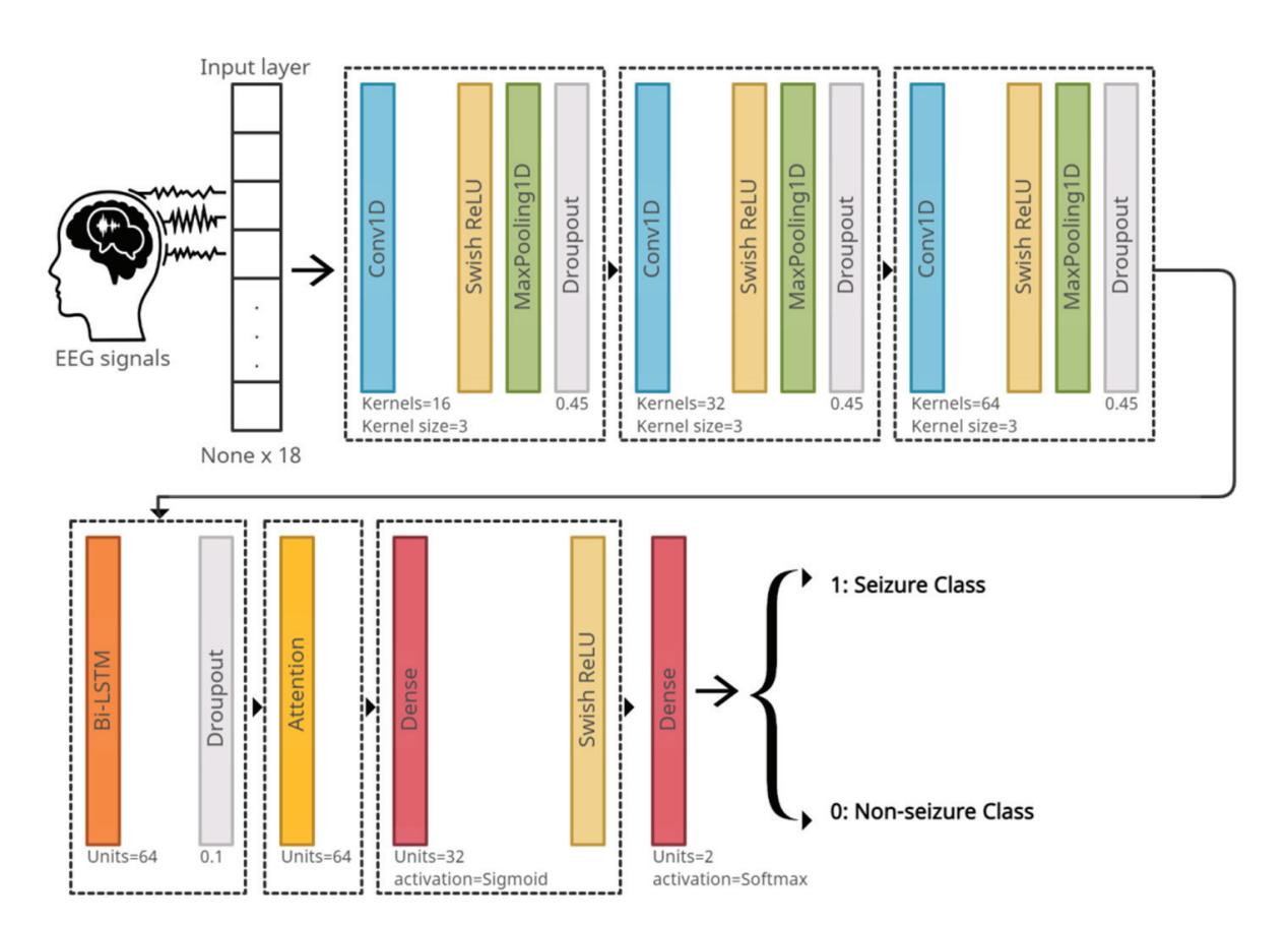
**Figure 5.** The deep-learning model architecture.
The loss function that is used in the proposed model is categorical cross-entropy. The adopted optimization algorithm for the model is the Adam algorithm [29]. One of the hyperparameters of the algorithm is the learning rate. The authors of Adam recommend setting the learning rate differently based on the system. It is better to use a decaying learning rate than a fixed one, which is a learning rate whose value decreases as the epoch number increases. This means it allows one to start with a relatively high learning rate while benefiting from lower learning rates in the final stages of training. This is useful where a relatively high learning rate is necessary to set huge steps, whereas increasingly smaller steps are necessary when approaching a minimum loss. The proposed model uses a learning rate with an initial value of 0.00001, taking into account the use of a common decay scheme, which allows learning rates to be dropped in smaller steps exponentially every few epochs.
#### 4.2. Seizure Detection Model
The proposed system is trained, validated, and tested on the CHB-MIT Scalp EEG dataset. It depends on the eighteen common channels that have been previously mentioned. The model suggested in Figure 5 is used, except each dropout layer is replaced by a batch normalization layer. The EEG signals are inputted to the system and passed through three CNN layers, each with different configurations as shown in Figure 5. Next are the Bi-LSTM and attention layers, respectively. Finally, the signals pass through two dense layers that classify the signal as seizure or non-seizure.
**Convolutional Neural Network:** The EEG signals are one-dimensional time series data; hence, for its analysis, a one-dimensional CNN is proposed (1D-CNN). The 1-D CNN automatically learns the discriminative features that represent the structure of EEG signals [30].
The activation function for the proposed model is the Swish Rectified Linear Unit (Swish Relu) [31]. The activation function's purpose is to classify and learn the non-linearity in the data. The formula for Swish Relu is as follows:
$$f(x) = x * sigmoid(\beta x)$$
(1)
where:
$$sigmoid(\beta x) = \frac{1}{1 + e^{-\beta x}}$$
(2)
16
*Sensors* **2022**, *22*, 6592
where β is a constant; if β is close to 0, the function will work linearly. If β is a large value, greater than or equal to 10, the function works similarly to Relu. After performing some experimental work, it is considered β = 1 in this study.
**Max Pooling:** Max-pooling 1D [32] is an operation which is usually appended to CNNs after the individual convolutional layers to down-sample the output. Max pooling is applied to reduce the resolution of the output of the convolutional layer, which decreases the network parameters and subsequently decreases the computational load as well as the overfitting. It is also helpful in selecting the higher valued frequencies as being the most activated frequencies. The filter (window) of size 3 is applied in the proposed system.
**Batch Normalization:** Throughout training, the distribution of the input data varies due to the update of the parameters. This will slow down the learning, so the learning becomes harder with nonlinearities. This phenomenon is called internal covariate shift [33]. To solve this issue, batch normalization is used. This makes the optimization significantly smoother, speeds up the training process, and slightly regularizes the model.
**Bidirectional Long Short-Term Memory:** Bidirectional LSTM (Bi-LSTM) [34] divides the standard LSTM's hidden neuron layer into two propagation directions: forward and backward. Therefore, this structure of Bi-LSTM will make it capable of processing the input in two ways: modeling from the front to the back and from the back to the front. The Bi-LSTM has the ability to detect the contextual information in long sequences of data and learn the importance of different events. For this purpose, the proposed system uses Bi-LSTM. In fact, the Bi-LSTM in the proposed model will make full use of the information before and after the states of epileptic seizure, enabling seizure events to be properly detected. The number of units of Bi-LSTM represents the dimensionality of the output space.
**Attention:** Attention [35] is the ability to highlight and use the salient parts of information dynamically in a similar way to the human brain. This type of mechanism works through iterative re-weighting to allow the model to utilize the most relevant components of the input sequence, which is the EEG signal, in a flexible manner in order to give these relevant components the highest weights. This type of mechanism was initially proposed and is usually used to process sequences such as EEG signals. For this reason, it was used in the proposed model. The Bi-LSTM with attention is a way to significantly enhance the model performance.
**Fully Connected Layer:** The fully connected layer [36] works as a classifier and predicts the input signal class. The proposed system has two dense layers. The first layer consists of thirty-two units (neurons), which represent the dimensionality of the output space. The second dense layer in the model has two units because the proposed model classifies the EEG signals into two classes: seizure or non-seizure. The reason for using two dense layers instead of one is that the convolution layers, in conjunction with the Bi-LSTM and attention layers, extract the features from the EEG signals. Depending on these features, the deep-neural network layers classify the signals. The first dense layer acts as a feature selector to decide whether or not a feature is relevant to a class, whereas the second dense layer acts as a classifier. Thus, the presence of two dense layers enhances the network's ability to better classify the extracted features.
#### 5. The Experimental Result
This section will be divided into two parts. The first one is to evaluate the compatibility framework for integrating local EEG data with the CHB-MIT dataset. The second one is to evaluate the seizure detection model.
17
*Sensors* **2022**, *22*, 6592
#### 5.1. Evaluating the Compatibility Framework
To assess the possibility of data integration, the DL model uses a set of well-known performance metrics to measure the model's performance: sensitivity, precision, and accuracy. The formulas for these metrics are shown below:
Sensitivity (Recall or Sen.) = $TP/(FN + TP)$ $(3)$
Precision (PRC) = TP/(TP + FP)
$$(4)$$
Accuracy (ACC) = (TP + TN)/(Total Samples)
$$(5)$$
where *TP* (True Positive) is the number of seizure signals that are detected as seizure, *FN* (False Negative) is the number of seizure signals that are detected as non-seizure, *TN* (True Negative) is the number of non-seizure signals that are detected as non-seizure, and *FP* (False Positive) is the number of non-seizure signals that are detected as seizure.
A set of experiments were performed to demonstrate the feasibility and usefulness of the deep-learning model for proving the concept of data integration and effectiveness of the compatibility framework with CHB-MIT dataset standards.
Initially, a random sample of EEG signals was taken from the CHB-MIT dataset for each experiment. Considering that the number of random EEG signals in the sample is proportional to the number of EEG signals extracted from the KAU dataset, the impact of KAU EEG signals can be studied by integrating them with the random sample. To clarify, the number of EEG signals extracted from the KAU dataset was 185 signals for both classes, and the number of random EEG signals in each sample was 750 signals. Therefore, the number of EEG signals from the KAU dataset constituted approximately 25% of the random sample size, which allows measuring the effectiveness of data integration. To illustrate, the number of EEG signals in each random sample from the CHB-MIT dataset was proportional to the number of EEG signals extracted from the KAU dataset in order to ensure that the impact of data integration from the KAU dataset with the CHB-MIT dataset was studied. The selection of signals in the sample was random to ensure that the effect of integration was properly studied. Therefore, multiple experiments were conducted with multiple random samples.
Six different experiments were performed as displayed in Table 5. Each experiment aims to measure the DL model performance on the sample extracted from the CHB-MIT dataset, and to merge the KAU EEG signals with a random sample also from the CHB-MIT dataset to study the effect of the data that is attached to the CHB-MIT dataset.
| EXP No. | DB | Avg. Epoch ACC | Avg. Epoch Sen.
for Seizure | Avg. Epoch Sen.
for No-Seizure | Avg. Epoch PRC
for Seizure | Avg. Epoch PRC
for No-Seizure |
|---------|---------------|----------------|--------------------------------|-----------------------------------|-------------------------------|----------------------------------|
| 1 | CHB-MIT | 79.25 | 64.16 | 93.14 | 89.2 | 75.29 |
| 2 | CHB-MIT | 81.93 | 68.43 | 94.41 | 91.54 | 78.03 |
| 3 | CHB-MIT | 75.38 | 54.95 | 94.02 | 89.26 | 70.53 |
| Avg. | CHB-MIT | 78.85 | 62.51 | 93.86 | 90 | 74.62 |
| 4 | CHB-MIT + KAU | 77.81 | 66.76 | 88.01 | 84.01 | 76.99 |
| 5 | CHB-MIT + KAU | 80.90 | 75.34 | 84.66 | 78.09 | 86.03 |
| 6 | CHB-MIT + KAU | 81.73 | 62.29 | 94.8 | 87.71 | 79.78 |
| Avg. | CHB-MIT + KAU | 80.15 | 68.13 | 89.16 | 83.27 | 80.93 |
**Table 5.** The performance of the DL model with and without data integration.
For further illustration, each random sample taken from the CHB-MIT dataset contained 750 random signals, which were then divided into training, validation, and testing at 50%, 20%, and 30%, respectively, so that the number of training signals was 375 and the number of testing signals was 225. It should be noted that the number of seizure signals was equal to the number of non-seizure signals in the first three experiments carried out
18
*Sensors* **2022**, *22*, 6592
on the CHB-MIT dataset only. The KAU EEG datasets were then randomly subdivided into training, validation, and testing groups. After that, these samples from KAU EEG data were merged with three random samples from the CHB-MIT dataset.
As noted in Table 5, the values of the performance metrics for each experiment before and after merging the random sample with the KAU EEG data are enhanced or within the same range, proving that the integration of data with the KAU dataset using the proposed framework is effective to combat the problem of data imbalance.
As seen, the proposed compatibility framework for creating a large and balanced dataset by integrating the EEG signals from the KAU dataset with the CHB-MIT dataset showed an improvement in the ability of the model to identify seizure signals with higher accuracy. The system suggested increasing the number of epilepsy signals and measuring the impact of integration on the performance of the model in terms of the overall accuracy of detecting epileptic seizures before and after the integration process. The overall accuracy of 78.85% increased to 80.15%. In particular, the performance improved through the sensitivity rate to epileptic seizures specifically; it was initially 62.51% and became 68.13%, meaning that the number of seizure signals that were detected as non-seizure was low, as reflected in the high sensitivity rate.
The model was trained on Google Colab using an Nvidia Tesla K80 GPU. Figure 6 shows the average values by epoch of the metrics that were previously mentioned in Table 5 for both classes of seizure and no-seizure. Through it, we note the high level of sensitivity after data integration which measures the percentage of seizure signals that were classified as seizure. However, we also observe from the chart that the level of precision slightly decreased after data integration which measures the proportion of no-seizure signals that were classified as no-seizure. The reason for this is the presence of artifact signals in the KAU dataset, which in turn were classified as seizure signals. This problem can be solved in future work by incorporating a tool into the model that deals with artifact signals. Finally, we notice an increase in overall accuracy after the data integration process, despite the decrease in precision, and the reason for this is the high sensitivity.
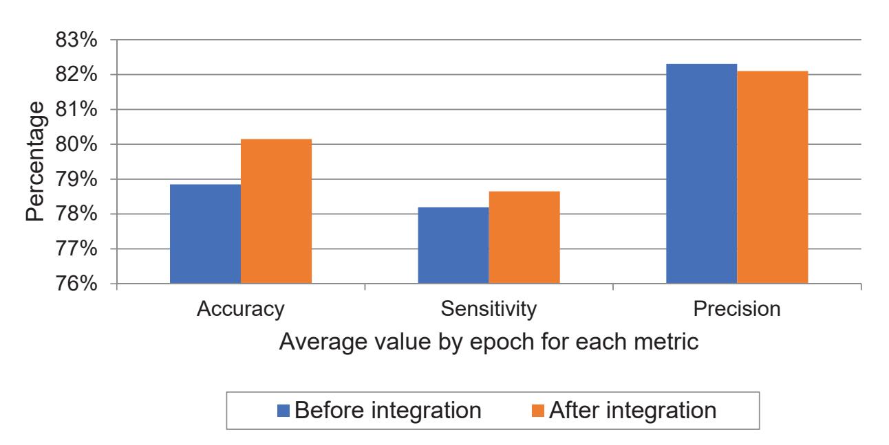
**Figure 6.** Average values of experiments before and after data integration for performance metrics.
#### 5.2. Evaluating the Seizure Detection Model
For evaluation and testing, 20% and 30% of the CHB-MIT dataset were used, respectively. The testing data constitutes about 12,000 windows of normal EEG records (no-seizure class) and about 3004 windows of epilepsy EEG records (seizure class). The performance was evaluated using the same performance metrics that are used to evaluate the compatibility framework, which are sensitivity, precision, and accuracy.
A comparison of the proposed model with state-of-the-art methods trained and tested on CHB-MIT is given in Table 6. As seen, the proposed system outperforms the previous systems, except for one [18] study. However, when we compare the proposed system with that study, we find that the study was only tested on 14 of the 23 patients in the dataset, but 19
*Sensors* **2022**, *22*, 6592
the proposed system was evaluated on all 23 patients. In addition, we find that although the algorithm for that study is patient-specific, its performance deteriorated significantly for patient 7, where the sensitivity rate reached 50%, because the duration of epileptic seizures for this patient was very short. This means that the algorithm works well if the duration of the seizure is long. However, if the seizure is brief, the accuracy drops dramatically. The proposed system provides good performance in both cases, whether the duration of the seizure is long or short, as seen through the sensitivity ratio of the proposed system, which was tested on all patients and overcame the sensitivity of the previous model.
| | | | Table 6. Performance comparison of the proposed model with other systems on the CHB-MIT dataset. |
|--|--|--|--------------------------------------------------------------------------------------------------|
|--|--|--|--------------------------------------------------------------------------------------------------|
| Cite | No. of Channels | No. of Subjects | Sen. | PRC | ACC | Speed of Convergence |
|--------------------|----------------------------------------|----------------------|-------|-------|-------|----------------------|
| [13] | 23 channels (in few
cases 24 or 26) | 23 | - | 96.51 | 96.61 | NA |
| [15] | 23 | 25% of the dataset | 91.15 | - | 95.11 | NA |
| [18] | 23 | 14 specific patients | 96.43 | - | 98.60 | NA |
| [19] | 23 channels (in few
cases 24 or 26) | 23 | 82.35 | - | 96.74 | Around 60 epochs |
| [21] | 23 channels (in few
cases 24 or 26) | 23 | 90.97 | - | - | NA |
| [20] | 23 channels (in few
cases 24 or 26) | 23 | 94 | - | 89 | NA |
| The proposed model | 18 channel | 23 | 96.85 | 96.98 | 96.87 | Around 130 epochs |
The uniqueness of the proposed deep-learning model lies in its design topology that suggests specific types of layers with specific configuration parameters, as in Figure 5, where the configuration of this model makes it capable of outperforming state-of-theart models by combining several advantages in the network design. First, it visually extracts the signal abnormalities from the 1D-EEG through the Conv1D, which is a visual neural network. Second, it learns the non-linearity in the EEG signals through swish Relu. Third, it identifies some distinct features from the higher valued frequencies as being the most activated frequencies through max-pooling. Fourth, it learns the seizure and no-seizure events from the contextual information before and after the states of epileptic or non-epileptic signals in forward and backward propagation directions through Bi-LSTM. Fifth, it improves the performance of the model significantly by combining attention with Bi-LSTM to give the relevant components the highest weights during the iterative re-weighting process.
Since the EEG patterns are highly subject-dependent, the main contribution of the proposed model is to deal with dual-detection problems (seizure versus non-seizure) based on using a small number of channels that are common for all patients, not for each patient separately, to achieve better performances than those of systems of full channels.
A limitation of the proposed model could be the inability to detect the seizure or no-seizure from the EEG signals with a sample rate of 512 Hz. For further improvement, the model can be trained using the decimate() method to down-sample the signal that has a sample rate of 512 Hz, which would enable the model to detect epileptic seizures from signals with a sampling rate of 256 or 512 Hz.
The model was trained on Google Colab using an Nvidia Tesla K80 GPU. Figure 7 shows the performance of the model by epoch for testing according to the metrics that were previously used in Table 6 for each class, seizure or no-seizure. We observe that the convergence of the model occurred at the 130th epoch. Comparing Kaziha et al. [19] with our model, our method shows a better sensitivity of 96.85% while theirs was 82.35%. One of the main reasons is that their window size was 100 s, whereas our window size was 10 s, which in turn takes only the exact seizure intervals.
20
*Sensors* **2022**, *22*, 6592
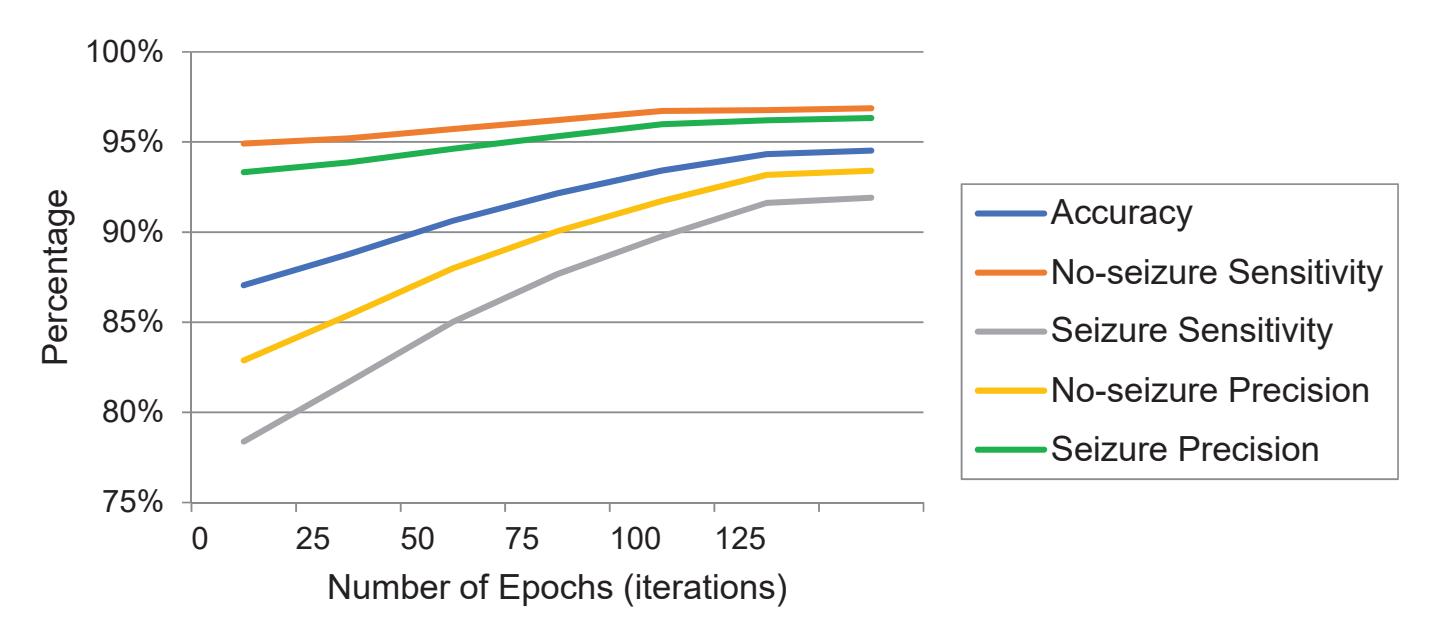
**Figure 7.** The performance metric charts of testing against the epochs.
#### 6. Conclusions
In this research, a compatibility framework for integrating local EEG signals into the CHB-MIT dataset is proposed. The proposed approach has multiple benefits. First, it overcomes the problem of data imbalance faced by most of the datasets in the field due to the low incidence of epileptic signals compared to non-epileptic signals. Second, it allows the establishment of large datasets by integrating local EEG signals with the available datasets required by the deep-learning models used to develop seizure detection and prediction systems. The approach presented in this paper can also be used as a support tool for researchers in the field to process and read local EEG signals that are of the XLtek type for which there were no reading functions available in the analysis software packages for such EEG types. In the end, a set of experiments carried out to examine the data integration using the proposed framework proved its feasibility and usefulness.
In addition, an automated epilepsy detection system that is based on some channels was proposed. This system deals with dual-detection problems (seizure versus nonseizure). The proposed system uses a wavelet decomposition technique and a simple one-dimensional convolutional neural network, along with bidirectional long-short-term memory and attention, to receive EEG signals as input data, pass them to various layers, and finally make a decision via a dense layer. This model can assist neurophysiologists to detect the seizures and significantly decrease the burden, while also increasing the efficiency.
There are several future suggestions regarding the proposed model. One such suggestion is that it could be incorporated into a wearable device for patients, considering the storage and memory requirements. Another suggestion is the possibility of deploying the system in a central cloud environment for rapid access via mobile devices without using specific wear-and-tear devices. The EEG signal that is considered as the input data is small in size and the proposed model is portable, which makes it appropriate for cloud deployment. The EEG signals are easily transferred to the cloud for processing in real-time as it can issue a warning alarm to notify the doctors/patients if needed. The proposed system can be used to implement expert systems for similar disorders that include EEG brain signals.
**Author Contributions:** Conceptualization, K.M.M., H.O.T. and M.K.A.; methodology, M.K.A. and K.M.M.; software, M.K.A.; validation, M.K.A., K.M.M. and D.M.A.; formal analysis, M.K.A.; investigation, M.K.A., K.M.M. and D.M.A.; resources, H.O.T.; data curation, M.K.A. and H.O.T.; writing original draft preparation, M.K.A.; writing—review and editing, M.K.A. and K.M.M.; visualization, M.K.A.; supervision, K.M.M. and D.M.A.; project administration, K.M.M. and D.M.A.; funding acquisition, D.M.A. All authors have read and agreed to the published version of the manuscript.
**Funding:** This research was funded by the Deanship of Scientific Research (DSR) at King Abdulaziz University, Jeddah, grant No. (D-1013-611-1443).
21
*Sensors* **2022**, *22*, 6592
**Institutional Review Board Statement:** The study was approved ethically by the Unit of Biomedical Ethics Research Committee at King Abdulaziz University Hospital, Jeddah, Saudi Arabia, on 6 January 2020 (Reference No. 3-20). The Unit of Biomedical Ethics is registered with the National Committee of Bio. & Med. Ethics (Registration No. HA-02-J-008).
**Informed Consent Statement:** Patient consent was waived due to the retrospective nature of the study and the analysis used anonymous clinical data.
**Data Availability Statement:** The CHB-MIT datasets analyzed during the current study are available in the PhysioNet repository [https://physionet.org/content/chbmit/1.0.0/ accessed on 10 August 2020]. While the KAU datasets that support part of the findings of this study are available from King Abdulaziz University Hospital, restrictions apply to the availability of these data, which were used under license for the current study, and so are not publicly available. Data is, however, available from the authors upon reasonable request and with permission of King Abdulaziz University Hospital.
**Acknowledgments:** We extend our sincere thanks to the Epilepsy Center at King Abdulaziz University Hospital for providing us with the local dataset to conduct the experiments and their cooperation throughout the study.
**Conflicts of Interest:** The authors declare no conflict of interest. The funders had no role in the design of the study; in the collection, analyses, or interpretation of data; in the writing of the manuscript; or in the decision to publish the results.
#### References
- 1. Panayiotopoulos, C. *A Clinical Guide to Epileptic Syndromes and Their Treatment*; Springer: Berlin/Heidelberg, Germany, 2010.
- 2. World Health Organization. Epilepsy. 2018. Available online: http://www.who.int/en/news-room/fact-sheets/detail/epilepsy (accessed on 20 August 2018).
- 3. Background to Seizures. Epilepsy Research UK. 2018. Available online: https://www.epilepsyresearch.org.uk/about-epilepsy/ background-to-seizures/ (accessed on 15 August 2018).
- 4. Bell, G.; Sinha, S.; Tisi, J.; Stephani, C.; Scott, C.; Harkness, W.; McEvoy, A.; Peacock, J.; Walker, M.; Smith, S.; et al. Premature mortality in refractory partial epilepsy: Does surgical treatment make a difference? *J. Neurol. Neurosurg. Psychiatry* **2010**, *81*, 716–718. [PubMed]
- 5. Ulate-Campos, A.; Coughlin, F.; Gaínza-Lein, M.; Fernández, I.; Pearl, P.; Loddenkemper, T. Automated seizure detection systems and their effectiveness for each type of seizure. *Seizure* **2016**, *40*, 88–101. [PubMed]
- 6. EEG (Electroencephalogram)—Mayo Clinic. 2022. Available online: https://www.mayoclinic.org/tests-procedures/eeg/about/ pac-20393875 (accessed on 3 August 2021).
- 7. Nacy, S.; Kbah, S.; Jafer, H.; Al-Shaalan, I. Controlling a Servo Motor Using EEG Signals from the Primary Motor Cortex. *Am. J. Biomed. Eng.* **2016**, *6*, 139–146.
- 8. Tatum, W.O. Ellen R. grass lecture: Extraordinary EEG. *Neurodiagnostic J.* **2014**, *54*, 3–21.
- 9. Birjandtalab, J.; Heydarzadeh, M.; Nourani, M. Automated EEGbased epileptic seizure detection using deep neural networks. In Proceedings of the 2017 IEEE International Conference on Healthcare Informatics (ICHI), Park City, UT, USA, 23–26 August 2017; pp. 552–555.
- 10. Buda, M.; Maki, A.; Mazurowski, M.A. A systematic study of the class imbalance problem in convolutional neural networks. *Neural Netw.* **2018**, *106*, 249–259. [CrossRef] [PubMed]
- 11. Shoeb, A. Application of Machine Learning to Epileptic Seizure Onset Detection and Treatment. Ph.D. Thesis, Massa-Chusetts Institute of Technology, Cambridge, MA, USA, 2009.
- 12. Antoniades, A.; Spyrou, L.; Took, C.C.; Sanei, S. Deep learning for epileptic intracranial EEG data. In Proceedings of the 2016 IEEE 26th International Workshop on Machine Learning for Signal Processing (MLSP), Vietri sul Mare, Italy, 13–16 September 2016; pp. 1–6.
- 13. Yuan, Y.; Xun, G.; Ma, F.; Suo, Q.; Xue, H.; Jia, K.; Zhang, A. A novel channel-aware attention framework for multi-channel EEG seizure detection via multi-viewdeep learning. In Proceedings of the 2018 IEEE EMBS International Conference on Biomedical & Health Informatics (BHI), Las Vegas, NV, USA, 4–7 March 2018; pp. 206–209.
- 14. Ullah, I.; Hussain, M.; Qazi, E.-U.-H.; Aboalsamh, H. An automated system for epilepsy detection using EEG brain signals based on deep learning approach. *Expert Syst. Appl.* **2018**, *107*, 61–71. [CrossRef]
- 15. Zabihi, M.; Kiranyaz, S.; Jantti, V.; Lipping, T.; Gabbouj, M. Patient-Specific Seizure Detection Using Nonlinear Dynamics and Nullclines. *IEEE J. Biomed. Health Inform.* **2019**, *24*, 543–555. [CrossRef] [PubMed]
- 16. Avcu, M.T.; Zhang, Z.; Chan, D.W.S. Seizure detection using least EEG channels by deep convolutional neural network. In Proceedings of the ICASSP 2019 IEEE International Conference on Acoustics, Speech and Signal Processing (ICASSP), Brighton, UK, 12–17 May 2019; pp. 1120–1124.
- 17. Hu, X.; Yuan, Q. Epileptic EEG Identification Based on Deep Bi-LSTM Network. In Proceedings of the 2019 IEEE 11th International Conference on Advanced Infocomm Technology (ICAIT), Jinan, China, 18–20 October 2019; pp. 63–66. [CrossRef]
*Sensors* **2022**, *22*, 6592
- 18. Chandel, G.; Farooq, O.; Khan, Y.; Varshney, Y. Patient Specific Seizure Onset-Offset Latency Detection using Long- term EEG Signals. In Proceedings of the 2019 International Conference on Electrical, Electronics and Computer Engineering (UPCON), Aligarh, India, 8–10 November 2019.
- 19. Kaziha, O.; Bonny, T. A Convolutional Neural Network for Seizure Detection. In Proceedings of the 2020 Advances in Science and Engineering Technology International Conferences (ASET), Dubai, United Arab Emirates, 4 February–9 April 2020.
- 20. Huang, C.; Chen, W.; Chen, M.; Yuan, B. A Feature Fusion Framework and Its Application to Automatic Seizure Detection. *IEEE Signal Process. Lett.* **2021**, *28*, 753–757. [CrossRef]
- 21. Jeong, S.; Jeon, E.; Ko, W.; Suk, H. Fine-grained Temporal Attention Network for EEG-based Seizure Detection. In Proceedings of the 2021 9th International Winter Conference on Brain-Computer Interface (BCI), Gangwon, Korea, 22–24 February 2021.
- 22. Holmes, G. Consequences of Epilepsy through the Ages: When is the Die Cast? *Epilepsy Curr.* **2012**, *12*, 4–6. [CrossRef]
- 23. Jadeja, N.M. Montages. In *How to Read an EEG*; Cambridge University Press: Cambridge, MA, USA, 2021; pp. 17–22.
- 24. Sharmila, A.; Geethanjali, P. DWT Based Detection of Epileptic Seizure From EEG Signals Using Naive Bayes and k-NN Classifiers. In Proceedings of the 2017 International Conference on Trends in Electronics and Informatics (ICEI), Tirunelveli, India, 11–12 May 2017; Volume 4, pp. 7716–7727. [CrossRef]
- 25. Zhang, T.; Chen, W.; Li, M. AR based quadratic feature extraction in the VMD domain for the automated seizure detection of EEG using random forest classifier. *Biomed. Signal Process. Control* **2017**, *31*, 550–559. [CrossRef]
- 26. Khan, Y.U.; Farooq, O.; Sharma, P. Automatic detection of seizure onset in pediatric EEG. *Int. J. Embed. Syst. Appl.* **2012**, *2*, 81–89. [CrossRef]
- 27. Akwei-Sekyere, S. Powerline noise elimination in biomedical signals via blind source separation and wavelet analysis. *PeerJ* **2015**, *3*, e1086. [CrossRef] [PubMed]
- 28. Frost, J. Z-score: Definition, Formula, and Uses. Statistics by Jim. 2022. Available online: https://statisticsbyjim.com/basics/zscore/ (accessed on 5 February 2022).
- 29. Kingma, P.D.; Ba, J.L. Adam: A method for stochastic optimization. *arXiv* **2017**, arXiv:1412.6980v9. [CrossRef]
- 30. Albawi, S.; Mohammed, T.A.; Al-Zawi, S. Understanding of a convolutional neural network. In Proceedings of the 2017 International Conference on Engineering and Technology (ICET), Antalya, Turkey, 21–23 August 2017; pp. 1–6. [CrossRef]
- 31. Ramachandran, P.; Zoph, B.; Le, Q.V. Searching for activation functions. *arXiv* **2017**, arXiv:1710.05941.
- 32. Murray, N.; Perronnin, F. Generalized Max Pooling. In Proceedings of the 2014 IEEE Conference on Computer Vision and Pattern Recognition, Columbus, OH, USA, 23–28 June 2014. [CrossRef]
- 33. Ioffe, S.; Szegedy, C. Batch normalization: Accelerating deep network training by reducing internal covariate shift. *arXiv* **2015**, arXiv:1502.03167.
- 34. Aggarwal, R. Bi-LSTM. *Medium*. 2019. Available online: https://medium.com/@raghavaggarwal0089/bi-lstm-bc3d68da8bd0 (accessed on 18 February 2022).
- 35. Verma, Y. A Beginner's Guide to Using Attention Layer in Neural Networks. *Analytics India Magazine*. 2022. Available online: https://analyticsindiamag.com/a-beginners-guide-to-using-attention-layer-in-neural-networks/ (accessed on 13 July 2022).
- 36. Unzueta, D. Convolutional Layers vs. Fully Connected Layers. Towards Data Science. 2021. Available online: https:// towardsdatascience.com/convolutional-layers-vs-fully-connected-layers-364f05ab460b (accessed on 20 February 2022).
23


*Article*
### A Classification Model of EEG Signals Based on RNN-LSTM for Diagnosing Focal and Generalized Epilepsy
**Tahereh Najafi 1, Rosmina Jaafar 1,\*, Rabani Remli 2 and Wan Asyraf Wan Zaidi 2**
- 1 Department of Electrical, Electronics and Systems Engineering, Universiti Kebangsaan Malaysia, Bangi 43600, Malaysia
- 2 Department of Medicine, Hospital Canselor Tuanku Muhriz, Universiti Kebangsaan Malaysia, Cheras, Kuala Lumpur 56000, Malaysia
- **\*** Correspondence: rosmina@ukm.edu.my
**Abstract:** Epilepsy is a chronic neurological disorder caused by abnormal neuronal activity that is diagnosed visually by analyzing electroencephalography (EEG) signals. Background: Surgical operations are the only option for epilepsy treatment when patients are refractory to treatment, which highlights the role of classifying focal and generalized epilepsy syndrome. Therefore, developing a model to be used for diagnosing focal and generalized epilepsy automatically is important. Methods: A classification model based on longitudinal bipolar montage (LB), discrete wavelet transform (DWT), feature extraction techniques, and statistical analysis in feature selection for RNN combined with long short-term memory (LSTM) is proposed in this work for identifying epilepsy. Initially, normal and epileptic LB channels were decomposed into three levels, and 15 various features were extracted. The selected features were extracted from each segment of the signals and fed into LSTM for the classification approach. Results: The proposed algorithm achieved a 96.1% accuracy, a 96.8% sensitivity, and a 97.4% specificity in distinguishing normal subjects from subjects with epilepsy. This optimal model was used to analyze the channels of subjects with focal and generalized epilepsy for diagnosing purposes, relying on statistical parameters. Conclusions: The proposed approach is promising, as it can be used to detect epilepsy with satisfactory classification performance and diagnose focal and generalized epilepsy.
**Keywords:** electroencephalography (EEG); epilepsy; long short-term memory (LSTM); theta frequency band; longitudinal bipolar montage (LB); signal processing; classification
**1. Introduction**
Epilepsy is a chronic disorder inducing subjects to experience seizures, leading to cognitive impairments, medical and psychiatric comorbidities, social stigmatization, and, in general, poor quality-of-life (QOL) [1]. A recent study reported that the prevalence of lifetime epilepsy was 7.8 per 1000 individuals in Malaysia in 2021 [2]. Diagnoses of epilepsy are basically clarified by an epileptologist based on a clinical assessment, neuro imaging, and the visual detection of interictal epileptiform discharges (IEDs) appearing in 30% of cases in their electroencephalography (EEG) signals [3]. EEG reveals a general overview of neuronal activity in disparate cortical regions by representing potential differences between certain areas of the brain and a determined reference on the head surface in timeseries data [4]. According to [5], known epilepsy is classified into two categories based on the clinical symptoms and the localization of manifested abnormalities in EEG. These epilepsy categories are focal epilepsy, which involves the partial region of the brain, and generalized epilepsy, which affects all regions of the brain. Although anti-seizure drugs (ASDs) are vastly used to control the number of seizures, about one-third of epileptic patients in the world are refractory to treatment, and surgical operation in which the epileptogenic foci need to be removed is the only option. As a result, detecting the affected area linked with
**Citation:** Najafi, T.; Jaafar, R.; Remli, R.; Wan Zaidi, W.A. A Classification Model of EEG Signals Based on RNN-LSTM for Diagnosing Focal and Generalized Epilepsy. *Sensors* **2022**, *22*, 7269. https://doi.org/ 10.3390/s22197269
Academic Editors: Yifan Zhao, Yuzhu Guo and Fei He
Received: 30 June 2022 Accepted: 20 September 2022 Published: 25 September 2022
**Publisher's Note:** MDPI stays neutral with regard to jurisdictional claims in published maps and institutional affiliations.

**Copyright:** © 2022 by the authors. Licensee MDPI, Basel, Switzerland. This article is an open access article distributed under the terms and conditions of the Creative Commons Attribution (CC BY) license (https:// creativecommons.org/licenses/by/ 4.0/).
*Sensors* **2022**, *22*, 7269. https://doi.org/10.3390/s22197269 https://www.mdpi.com/journal/sensors
24
*Sensors* **2022**, *22*, 7269
the seizure onset zone plays a pivotal role in the process of treatment [6]. The challenge to the diagnosis phase mostly arises from the need to assess long-term EEG recordings, which is time-consuming and prone to inaccuracy due to human error. Consequently, training models for IED observation may be useful in the diagnosis process, especially at times when an epileptologist is unavailable.
Literature shows that the focus in the majority of epilepsy studies is summarized in seizure detection using machine or deep learning techniques to determine the type of epilepsy [7]. This study is concentrated on interictal duration and in the cases in which IEDs are not necessarily available. Diagnosing different types of epilepsy does not solely depend on analyzing EEG signals for discovering IEDs. In this regard, machine learning techniques are used in analyzing epileptic EEG signals. The analysis comprises the following main steps: pre-processing, feature extraction and classification.
Feature extraction of machine learning technique is done in time, frequency, or time– frequency domains [8]. Time–frequency methods such as flexible analytic wavelet transform [9,10], short-time Fourier transform [11], discrete wavelet transform (DWT) [12], Hilber Huang transform [13], and empirical mode decomposition [14] have been considered for diagnosing epilepsy. Automatic focal and non-focal epilepsy were detected using entropy-based features from flexible analytic wavelet transform in [10]. Wavelets, scatter matrices, and quadratic classifiers were, respectively, employed for feature extraction, feature dimensionally reduction, and classification in [15] in order to classify EEG signals to detect epileptic seizures. The study reached a 99% accuracy in distinguishing healthy controls from subjects with epilepsy, with or without seizures. An interictal seizure-free period has been analyzed by [16] using triggering signals of intermittent photic stimulation (IPS) reporting frequency domain features; the theta band is the most fitting feature in diagnosing generalized epilepsy in the visual cortex. This classification has been done with a support vector machine (SVM) in 18 Hz IPS, reaching the best discrimination between groups. The authors in [17] in 2017 introduced a statistical-based solution to overwhelm the empirical or arbitrarily determination of the level of decomposition in wavelets. The study reached an accuracy of more than 80% in detection using an SVM for two datasets: Bern Barcelona and University of Bonn. The authors in [18] evaluated different wavelet families using a probabilistic neural network (PNN) and an SVM. The study reported Coiflet as the best wavelet family in diagnosing epilepsy. Literature shows that the SVM is a valuable tool and is vastly used as a valuable classifier in a variety of clinical diagnostic research [19].
After feature extraction, feature dimensionality reduction is a vital step in analyzing signals in cases where we want to reduce irrelevant features and determine the most effective ones with a high model performance. This can be done through various methods such as feature selection or a combination of features, both of which rely on mathematical solutions behaving as filters, wrappers, and embedded strategies [20,21]. Detecting epileptic seizures with a focus on feature selection based on fuzzy membership was achieved in [22]. The authors in [23] conducted a comparative study to analyze discriminative features using various feature selection techniques in epilepsy. A method for EEG feature selection was introduced in [24] via stacked deep embedded regression with joint sparsity.
Classification steps have been taken by a variety of linear and non-linear classifiers, such as the decision tree [25], logistic regression [26], the k-nearest neighbor, the support vector machine [27], Naive Bayes [28], and artificial neural networks [29–31], or deep learning [32]. Artificial intelligence encompasses a variety of areas, and one of them is deep learning (DL). Before the rise of DL, conventional machine learning algorithms involving feature extraction were used. Their performance was limited to the ability of those handcrafting the features. However, in DL, the extraction of features and classification are entirely automated. These techniques have made significant advances in many areas of medicine, such as in the diagnosis of epileptic seizures.
The drawback of machine learning algorithms, albeit still beneficial, is that their performance is limited to the ability of those handcrafting the features [33]. Artificial intelligence encompasses a variety of areas, and one of its branches is deep learning. The 25
*Sensors* **2022**, *22*, 7269
priority of deep learning compared to machine learning is that the extraction of features and classification are entirely automated. The paper cited above comprehensively revies deep learning techniques in epilepsy studies from 2016 to 2021 using EEG and neuroimaging techniques with a focus on seizure detection. The review represented the available epilepsy datasets, such as Freiburg, CHB-MIT, and Bonn. It was reported that the majority of researchers employed their own clinical dataset. With a focus on EEG and epilepsy, the paper represented the definition of some of the high-usage deep learning models: onedimensional convolutional neural networks (1D-CNNs), recurrent neural networks (RNNs) and two of its branches, long short-time memory (LSTM) and gated recurrent units (GRUs), autoencoders (AEs), CNN-RNNs, and CNN-AEs. The paper collected 24 papers on EEG signals in epilepsy detection using 1D-CNNs. The studies used 4–33 layers for their models and found diagnosis accuracies ranging from 79.34% to 99.28% (with one reaching 100%) using mostly Softmax and in some cases SVM classifiers. In 15 studies that applied an RNN and its different branches, mainly LSTM, the accuracy reported was superior (from 84.35% to 98.91% and one 100%) to the CNN. The papers mostly used 4 layers (minimum 3, maximum 48 layers) for their models and mainly used using Softmax and Sigmoid, with one study using multilayer perceptron (MLP) classifiers.
An RNN is developed to process timeseries data through cyclic connections based on feedforward neural networks. The method has been vastly used for seizure prediction with classification approaches. The history of input in an RNN is mapped in order to predict each output by weighting the temporal relationships between the data at each time point. The issue is that a vanishing gradient problem causing the given input influences hidden and output layers, thus decaying or exploding exponentially over time [34]. One of the popular solutions for this is to use LSTM. RNN-LSTM consists of connected subnetworks called a memory block, which remembers inputs for a long time. The authors in [35] used a combination of a 1D-CNN and LSTM for epileptic seizure detection. The authors in [36] investigated the automatic detection of epilepsy by a CNN-LSTM using the University of Bonn dataset and reached an accuracy of more than 80%. CNN-LSTM was further used in [37] on the same dataset to detect epileptic seizures, approaching a 99.71% accuracy, with a focus on the Tunable-Q Wavelet Transform (TQWT) in feature extraction. Using time series data and LSTM to analyze sequenced data, the authors in [38] were able to introduce a hybrid model by a dense convolutional network and LSTM using information transferred from DWT to images for prediction purposes.
In the present study, a model using RNN-LSTM is proposed for distinguishing normal subjects from subjects with epilepsy without observing IEDs. The model is further validated by correctly diagnosing focal and generalized epilepsy. Hence, retrospective EEG data from normal subjects and patients with focal and generalized epilepsy were used. The data of normal subjects and focal epilepsy patients were used for classification purposes, whereas the data of focal and generalized epilepsy patients were used for validating our classification model. After pre-processing using DWT, a longitudinal bipolar (LB) montage was calculated for all groups. Next, features were extracted in time and frequency domains for further selection based on *p*-values of Pearson's linear correlation coefficient. Signals were segmented, and the network was trained by a sequence of selected features extracted from each segment. Instead of raw signals, we used features extracted from segments as sequenced data to feed the network. The optimal group of features and the best model are employed to diagnose focal and generalized groups via classifying their LB channels as epileptic or normal, as depicted in Figure 1. The findings reveal that the proposed classification model is effective in detecting epileptic signals from normal signals and diagnosing focal and generalized epilepsy.
26
*Sensors* **2022**, *22*, 7269
**Figure 1.** A flowchart of the study.
#### 2. Materials and Methods
#### 2.1. Dataset
In this study, two sets of data were used for two purposes: to train the classification model (classification approach) and to validate the model (diagnosing approach). EEG data were collected from the hospital Canselor Tuanku Muhriz (HCTM) in Cheras, Malaysia. In the classification approach, the focus is classification between normal and epileptic subjects. In this regard, the temporal lobe channels of 42 patients suffering from nonlesional temporal lobe epilepsy (TLE) and the temporal lobe channels of 62 normal subjects were used. In the diagnosing approach, i.e., distinguishing between focal and generalized epilepsy, whole EEG channels of 50 patients with generalized epilepsy and whole EEG channels of 42 TLE patients were used. Some generalized patients had a normal EEG and were diagnosed as generalized epilepsy patients based on clinical symptoms. EEG was recorded from Fp1, Fp2, F3, F4, F7, F8, C3, C4, P3, P4, T3, T4, T5, T6, O1, and O2: a total of 16 electrodes via the Nicolet EEG device based on the 10–20 EEG standard electrode placement system for each case. For the measurement of EEG signals, subjects (male and female; age: 36.90 ± 13.40) were prepared to contain a contact impedance of less than 5 kΩ and recorded at a 500 Hz sample rate, and data recording was done during a resting state. The affected channels in the TLE cases were deemed as the epilepsy group, and the
27
*Sensors* **2022**, *22*, 7269
same channels in the normal cases were deemed as the normal group. From EEG reports and patients' clinical profiles, we determined that the placements of the affected channels were identified by neurologists in the inferior, mid, and superior areas of the temporal gyrus, i.e., in the right, left, or both hemispheres reflected in specific EEG channels under LB montage: Fp1-F7, F7-T3, T3-T5, T5-O1, Fp2-F8, F8-T4, T4-T6, and T6-O2. The affected channels were referred to as the channels with epilepsy localization. Therefore, the montage was calculated for 10 s of all datasets, 51 affected channels were identified as the epilepsy group, and 62 channels of the same regions were considered as the normal group. This data were studied to train our network. In the final stage, the classification model was validated by testing all LB channels from 50 generalized patients and the same 42 TLE patients (lateralized TLE and both hemispheres affected). The classification model and all EEG analysis were implemented via MATLAB (R2020a).
#### 2.2. Pre-Processing
Pre-processing focused on signal preparation in the aspect of eliminating artifacts due to muscular movement and blinking as well as swallowing manually. DWT using coif3 from the Coiflet family was applied to 10 s of raw signals for both the epileptic and the normal groups to eliminate power line noise by three levels of signal decomposition [39]. A longitudinal bipolar montage was calculated for each group by subtracting the amounts of potential differences between pertinent electrodes [40]. Figure 2 demonstrates the LB montage and the calculation details. In the figure, the cross mark represents the placement of the reference (Ref) while recording EEG signals—somewhere between the frontal lobe and central sulcus. LB consists of 18 channels; in this study, only 16 channels in the left and right posterior and anterior regions were calculated, and the leads Fz, Cz, and Pz were ignored.
| Left Posterior | Left Anterior | Right Anterior | Right Posterior |
|----------------------|----------------------|----------------------|----------------------|
| Fp1-F7: | Fp1-F3: | Fp2-F4: | Fp2-F8: |
| (Fp1-Ref) - (F7-Ref) | (Fp1-Ref) - (F3-Ref) | (Fp2-Ref) - (F4-Ref) | (Fp2-Ref) - (F8-Ref) |
| F7-T3: | F3-C3: | F4-C4: | F8-T4: |
| (F7-Ref) - (T3-Ref) | (F3-Ref) - (C3-Ref) | (F4-Ref) - (C4-Ref) | (F8-Ref) - (T4-Ref) |
| T3-T5: | C3-P3: | C4-P4: | T4-T6: |
| (T3-Ref) - (T5-Ref) | (C3-Ref) - (P3-Ref) | (C4-Ref) - (P4-Ref) | (T4-Ref) - (T6-Ref) |
| T5-O1: | P3-O1: | P4-O2: | T6-O2: |
| (T5-Ref) - (O1-Ref) | (P3-Ref) - (O1-Ref) | (P4-Ref) - (O2-Ref) | (T6-Ref) - (O2-Ref) |
**Figure 2.** Longitudinal bipolar montage calculation separated in the left and right posterior and anterior areas.
LB calculation is defined by replacing targeted leads, as shown by arrows in Figure 2, with the original reference during the EEG recording. For instance, for calculating Fp1-F7 as the first LB channel, first the potential difference recorded from both leads must be added by the amount of the original Ref. The new F7 should then be considered as the new reference for Fp1. This means that the value of F7 must be subtracted from the value of Fp1. In this study, due to the deficiency of the original Ref value, this amount was considered as a common subtracted value in LB calculation. Figure 3 represents 10 s of normal and epileptic EEG signals from one LB channel in the temporal region. Figure 4 exhibits a sample of de-noised generalized and TLE EEG data based on an LB montage.
28
*Sensors* **2022**, *22*, 7269
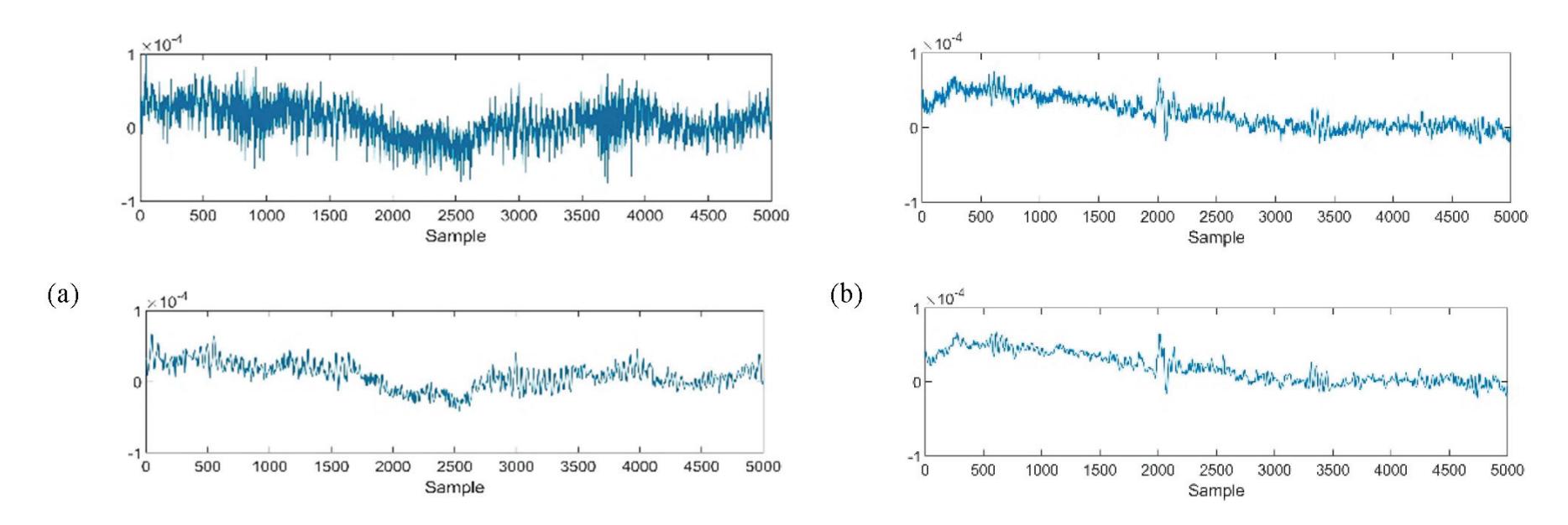
**Figure 3.** Samples of raw signals (top) and de-noised signals (down) of normal (**a**) and epileptic (**b**) signals recorded from T4−T6. The X-axis shows the potential difference (μv).
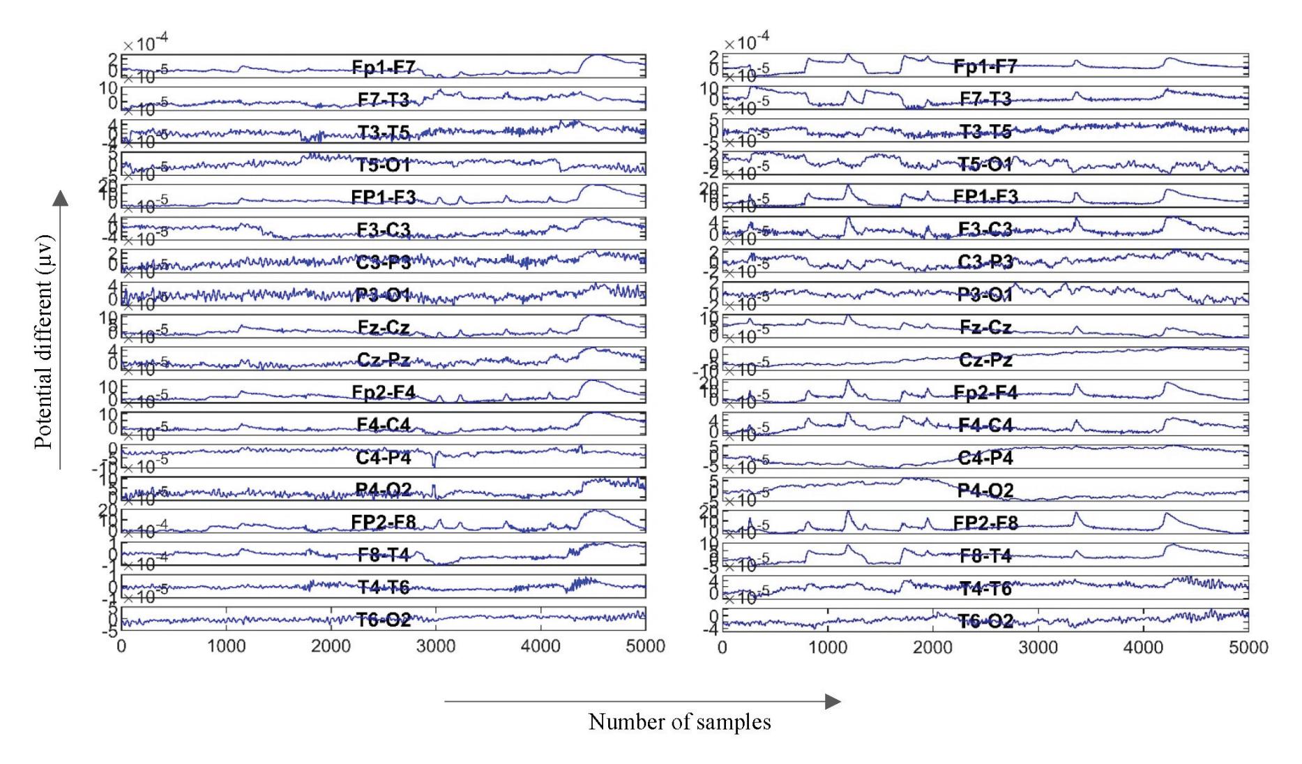
**Figure 4.** Generalized epilepsy (**left**) and TLE (**right**) samples based on the LB montage.
#### 2.3. Feature Extraction
Fifteen features in the time and frequency domains were extracted from each channel of both the epileptic and normal group: mean, standard deviation (STD), peak-to-peak (P2P), min, max, skewness (Skew), kurtosis (Kurt), peak-to-root sum square (P2RMS), root sum square (RSS), power of delta frequency band (delta; 1–4 Hz), power of theta frequency band (theta; 4–8 Hz), power of alpha frequency band (alpha; 8–14 Hz), power of beta frequency band (beta; 14–30 Hz), and power of gamma frequency band (gamma; over 30 Hz). Figure 5 exhibits a sample of the power spectrum density for one epileptic channel and one normal channel.
29
*Sensors* **2022**, *22*, 7269
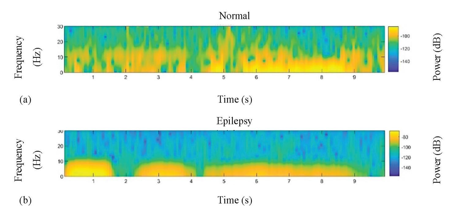
**Figure 5.** A Sample of power spectral density for one normal channel (**a**) and one epileptic (**b**) channel.
#### 2.4. Feature Selection
Pearson's rank correlation coefficients between all pairs of variables were calculated. The hypothesis test was considered in order to determine which correlations are significantly different from zero. Features with *p*-value <0.05, i.e., theta, alpha, beta, mean, min, skew, and kurt, were considered if they show a high classification performance. In addition, the features with the lowest correlation (≤20%) were considered, and the features with a high correlation (≥80%) were added separately to the group. Therefore, three groups of five features with low correlations were considered to feed the network.
#### 2.5. Classification Model Using RNN-LSTM
In this research, we used the RNN-LSTM architecture to identify epilepsy and diagnose focal and generalized epilepsy. Hence, the network was implemented with five layers: a sequence input layer, a bidirectional LSTM (BiLSTM) layer with 200 hidden units, a fully connected layer, a SoftMax layer, and a classification output layer. Table 1 represents the details of deep learning layers, values, and descriptions for training the network. The network is fed based on 10-fold cross validation achieved by 80% of the data for training and the remaining 20% was used for testing. EEG signals were segmented with 50% overlapping—1 s for each. Three groups of features were extracted from each segment. The model was trained by each group of features. The model with the best performance was considered as our classification model. In the next stage of the study, the classification model was applied to all LB channels of the focal and generalized epilepsy groups. The overall value of infections for each channel for each group was then calculated, separately. The variance of the overall values, which shows that the channel is affected, was measured for each channel of both groups. A high variance indicates that some channels are affected more than others by our model. Focal and generalized epilepsy cases were encountered when features had high and low variance; respectively. This was used as to validate our classification model.
**Table 1.** Deep learning layers and network training options.
| Deep learning Layers | Value | Description |
|----------------------|------------------------------|-------------------|
| BiLSTMLayer | BiLSTM with 200 hidden units | Output Mode: Last |
| FullyConnectedLayer | 2 fully connected layers | |
| SoftmaxLayer | Softmax | |
| ClassificationLayer | Crossentropyex | |
30
*Sensors* **2022**, *22*, 7269
**Table 1.** *Cont.*
| Training Option | Value | Description |
|-------------------|-------|--------------------------------------------------------------------------------------|
| ADAM | - | Adoptive moment estimation—Optimization Algorithm |
| MaxEpochs | 30 | 30 passes through the training data in the network |
| MiniBatchSize | 150 | Leads the network to look at 150 training signals at a time |
| InitialLearnRate | 0.01 | Assists to speed up the training process |
| GradientThreshold | 1 | To stabilize the training process by preventing gradients
from becoming too large |
#### 3. Results and Discussion
#### 3.1. Classification Approach
Figure 6a shows the significance level for the correlation tests specified as a scalar between 0 and 1, representing a low or high correlation, respectively. Negative values show a negative correlation among the relevant features. The figure shows the correlation between two features in the group. As shown, there are three strong correlated group of features surrounded by red boxes that need to be chosen individually, while the rest in these boxes are dropped out [41]. In addition, there are seven features where *p* < 0.05, i.e., theta, alpha, beta, mean, min, skew, and kurt, indicating significant features for discrimination (Figure 6b). In addition, a high correlation between the power of frequency bands restricted us from introducing three groups of features separated by theta, alpha, or beta. Therefore, we will have three groups of features with theta, alpha, and beta added separately to the mean, min, skew, and kurt.
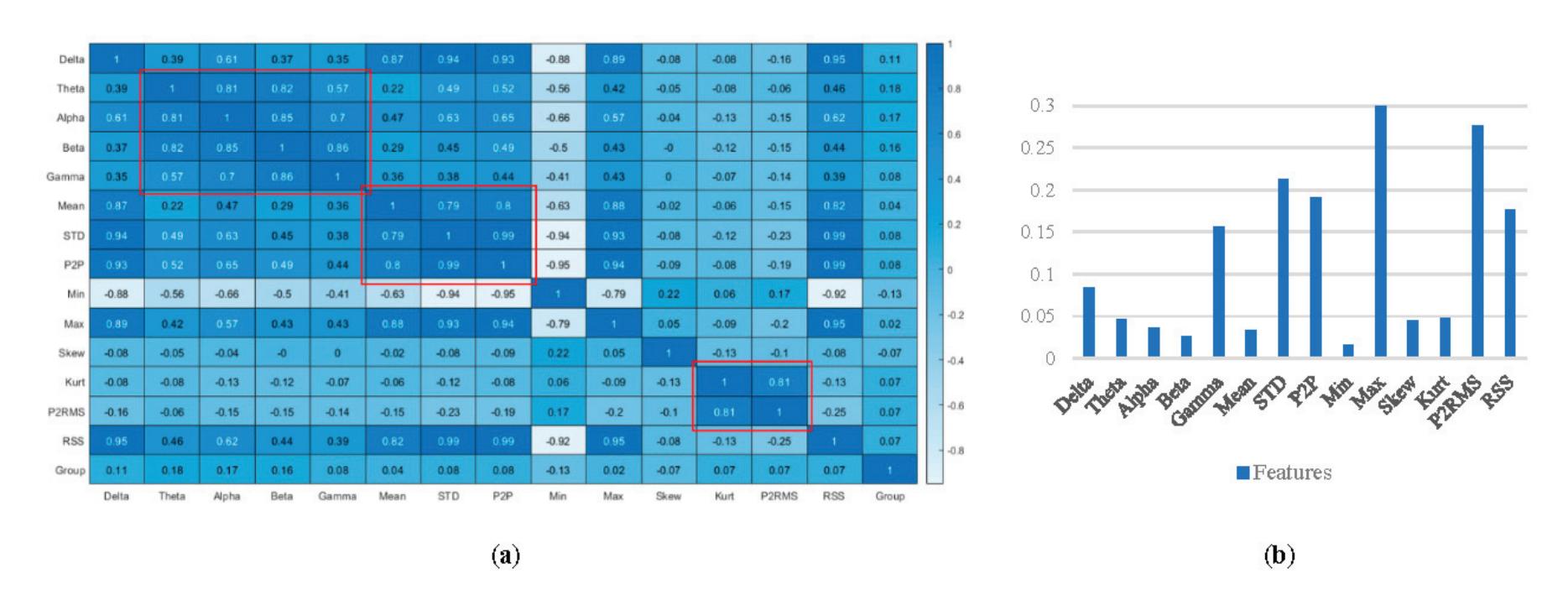
**Figure 6.** Correlation coefficient among features (**a**), *p*-value for each feature in group (**b**).
The ability of the model performance for discrimination has been characterized by sensitivity, specificity, accuracy, positive predictive value (PPV), and negative predictive value (NPV), referring to Equations (1)–(5), respectively. The sensitivity presents the percentage of detecting case subjects, while specificity emphasizes the ability to detect normal subjects. The accuracy is the amount of total detection for both patients and normal subjects from the study population. PPV and NPV represent the proportion of subjects with a positive test result who actually have the disease and those with a negative result who do not have the disease, respectively.
Sensitivity =
$$\frac{TP}{TP + FN} \times 100$$
(1)
31
*Sensors* **2022**, *22*, 7269
Specificity =
$$\frac{TN}{TN + FP} \times 100$$
(2)
$$Accuracy = \frac{TP + TN}{TN + FP + TP + FN} \times 100 \quad (3)$$
PPV = $\frac{TP}{TP + FP}$ \times 100
(4)
$$NPV = \frac{TN}{FN + TN} \times 100$$
where TP is true positive, representing patients that were correctly diagnosed among the patients, TN is true negative, indicating the number of normal subjects that were correctly diagnosed among normal subjects, FN is false negative, showing the number of subjects wrongly diagnosed as normal among the patients, and FP is false positive, representing the number of subjects wrongly diagnosed as patients among the normal subjects. Table 2 presents the network performance for three groups of features. It seems that the discrimination ability using the first group, highlighted in the table, is higher than the rest. Table 3 shows the details of the confusion matrix for three groups of selected features. The table shows that the model can detect epilepsy well, but there is still some confusion in detecting some samples. The model based on the features of Group 1 incorrectly detected three samples as epileptic instead of normal, and it detected only one normal sample as epileptic. Similarly, with the features of Group 3, there were significantly more false negatives than there were false positives. In contrast, the features of Group 2 led to the opposite balance, where the number of normal samples detected as epileptic was slightly higher. In general, the model behaved better using the features of Group 1, with emphasis on the power of the theta frequency band.
**Table 2.** The performance of the network in distinguishing normal subjects from epileptic subjects in the training stage.
| Groups of Features | Acc (%) | Sen (%) | Spc (%) | PPV (%) | NPV (%) |
|---------------------------------------|---------|---------|---------|---------|---------|
| Group 1: mean, min, skew, kurt, theta | 96.1 | 96.8 | 97.4 | 98.4 | 92.7 |
| Group 2: mean, min, skew, kurt, alpha | 90.4 | 94.0 | 85.4 | 91.0 | 89.7 |
| Group 3: mean, min, skew, kurt, beta | 91.4 | 87.3 | 97.6 | 98.0 | 82.0 |
**Table 3.** The details of the confusion matrix for the three groups of features.
| Actual
Classes | | Predicted Classes | | | | | |
|-------------------|----|-------------------|--------|-----------|--------|-----------|--------|
| | | Group 1 | | Group 2 | | Group 3 | |
| | | Epileptic | Normal | Epileptic | Normal | Epileptic | Normal |
| Epilepsy | 38 | 1 | 35 | 6 | 40 | 1 | |
| | 3 | 62 | 4 | 59 | 8 | 55 | |
#### 3.2. The Diagnosing Approach
The classification model was applied to each LB channel of EEG recordings from subjects with generalized and focal epilepsy. Figure 7 illustrates the result of the classification model for both groups by presenting the percentage of affected channels in the left or right posterior or anterior LB montage. Regarding focal epilepsy, the majority of the left and right posterior LB channels were diagnosed as affected in over 60% of the study population. Moreover, in the same group, all anterior LB channels were classified as affected in approximately 50% of the study population. In contrast, the generalized epilepsy findings indicate that affected LB channels were affected at a slightly constant rate in approximately 50% of its population. The average (55.59%) and variance (272.14) of detection for focal epilepsy, and the average (44.01%) and variance (51.05) of detection for
*Sensors* **2022**, *22*, 7269

generalized epilepsy, validate the classification model as a promising tool for distinguishing epileptic signals from normal signals without analyzing IEDs.
**Figure 7.** The result of the classification model for focal (blue) and generalized (grey) groups in classifying each channel as affected channels. The X-axis represents LB channels categorized in the left and right posterior and anterior areas. The Y-axis represents the percentage of affected channels according to the population of each group.
Figure 7 appears to indicate that the temporal lobe is not the only region affected in TLE, and the frontal area may be involved in this type of epilepsy. TLE is associated with long-term memory dysfunction [42]. The frontal lobe is related to cognition comprising executive skills as well as memory [43]. Evidence from neurophysiological and neuroimaging literature confirms the deficiency in executive function in the frontal lobe and working memory in TLE cases. The facts support this part of our study achievement.
Turning back to feature extraction step, the power of the theta frequency band were more effective in the classification model compared to the alpha and beta frequencies, albeit being accompanied with four other features (mean, min, skew, and kurt). There is an assumption that epilepsy characteristics are related to theta band connectivity in patients suffering from epileptic seizures [44]. A systematic review confirmed a consistent association between the theta frequency band and idiopathic epilepsy [45]. The authors in [46] reported an increment in theta activity during resting states in patients with major epilepsy syndromes. A diagnostic epilepsy study worked on the spectral power of different frequency bands in controls, patients with well controlled idiopathic generalized epilepsy, and drug-resistant patients. The study confirmed a higher interictal EEG spectral power in all frequency bands, and the reported frequency band were useful in diagnosing epilepsy.
Furthermore, the hippocampus has been claimed as the main structure involved in generating theta oscillations [47]. In 2021, the authors in [48] assessed the effects of hippocampal stimulation by inducing theta frequency, resulting in convulsion elimination. The authors in [49] conducted a successful animal study using deep brain stimulation (DBS) in attenuating seizures in TLE. The hypothesis was the reversal of the effects of stimulation augmentation of the hippocampal theta oscillation. Moreover, it was reported that epileptic seizures occur less often during waking periods or paradoxical sleep period and in conditions when the hippocampal theta rhythm can be observed.
#### 4. Conclusions
In this work, we defined two approaches in proposing a classification model for detecting epilepsy. The first approach was an essential one (the classification approach), and the second approach (the diagnosing approach) was focused on using the model to diagnose focal and generalized epilepsy using statistics. In the classification approach, 33
*Sensors* **2022**, *22*, 7269
brain signal processing techniques were implemented for signal pre-processing. De-noising signals and discovering affected channels were performed via DWT and LB montage calculation, respectively. Feature extraction was performed using methods in the time and frequency domains. Feature selection was performed using correlation coefficients. Classification was performed using RNN-LSTM. In this approach, the first aim is to find optimal features in distinguishing epileptic subjects from normal subjects, whereas the second aim is to extract features from segmented EEG signals. Continuous features are fed to the network. In the diagnosing approach, the best classification model was used for each LB channel of focal and generalized epilepsy subjects. The variance of the overall affected channels represented the type of epilepsy, where a high and low variance refers to focal and generalized epilepsy, respectively. In this work, three groups of EEG data were considered: normal subjects (non-epilepsy) and subjects with focal (TLE) and generalized epilepsy. Affected channels were collected from subjects without epilepsy and with focal epilepsy using the classification approach, whereas subjects with focal and generalized epilepsy were considered in the diagnosing approach. The results show that the best classification model was achieved through employing mean, min, skewness, kurtosis, and the power of the theta frequency band, with 96.70% accuracy, 94.44% sensitivity, and 97.6% specificity. Furthermore, it seems that the theta frequency band was more successful than alpha and beta in the detection procedure. The results show a remarkable difference in variance in the diagnosing approach via the proposed classification model. The most important limitation here is the potential lack of IEDs in epileptic EEG signals during interictal periods. Therefore, confident affected signals according to EEG reports were considered as a reference for training network. Furthermore, we could not test the model for other different types of focal lobe epilepsy due to the lack of data caused by a lower prevalence. In our study, we used affected signals from TLE cases because TLE is significantly prevalent in the HCTM dataset. TLE is also known as one of the most common causes of focal epilepsy and one of the most frequent indications of epilepsy surgery. Therefore, TLE became the only option for checking the validity of the model in the diagnosing approach. There is a thread to validate in the classification stage. Despite the selected features that significantly distinguished epileptic subjects from normal subjects, the validation may become confronted with a lower variance in diagnosing focal versus generalized epilepsy by increasing the amount of data. In future work, investigation on more data is suggested. Moreover, it would be beneficial not to combine both hemispherical focal epilepsy in the same diagnosing process. The model then might be needed to optimize the internal parameters that indicate the affected hemisphere.
**Author Contributions:** The paper is prepared by collaboration among authors in different aspects. The original draft preparation, conceptualization, methodology, software, formal analysis, in-vestigation and visualization were done by T.N. Conceptualization, resources, review and editing, supervision, project administration as well as funding acquisition were done by R.J., R.R. and W.A.W.Z. were responsible for validation, resources and data curation. All authors have read and agreed to the published version of the manuscript.
**Funding:** This research was funded by the Ministry of Higher Education Malaysia through the Fundamental Research Grant Scheme (FRGS/1/2019/TK04/UKM/02/3). The APC was funded by the same grant in addition to two internal grants received from Faculty of Engineering and Built Environment, UKM (DPP-2022 and TAP-20030).
**Institutional Review Board Statement:** The study was conducted in accordance with the Declaration of Helsinki, and approved by the Universiti Kebangsaan Malaysia Ethics Committee (UKM PPI/111/8/JEP-2021-177), date of approval on 19 April 2021.
**Informed Consent Statement:** Patient consent was waived due to collective report on the overall study results based on retrospective data. This adheres to the research ethics approval.
**Data Availability Statement:** The data used in the study are not publicly available as the data repository belongs to HCTM that bounds to the ethics approval.
34
*Sensors* **2022**, *22*, 7269
**Acknowledgments:** The authors would like to thank the Ministry of Higher Education Malaysia for funding the research and UKM Research Ethics Committee for the ethics approval.
**Conflicts of Interest:** The authors declare no conflict of interest.
#### References
- 1. Vaurio, L.; Karantzoulis, S.; Barr, W.B. The Impact of Epilepsy on Quality of Life. In *Changes in the Brain*; Springer: New York, NY, USA, 2017; pp. 167–187.
- 2. Fong, S.-L.; Lim, K.-S.; Tan, L.; Zainuddin, N.H.; Ho, J.-H.; Chia, Z.-J.; Choo, W.-Y.; Puvanarajah, S.D.; Chinnasami, S.; Tee, S.-K.; et al. Prevalence study of epilepsy in Malaysia. *Epilepsy Res.* **2021**, *170*, 106551. [CrossRef] [PubMed]
- 3. Renzel, R.; Tschaler, L.; Mothersill, I.; Imbach, L.L.; Poryazova, R. Sensitivity of long-term EEG monitoring as a second diagnostic step in the initial diagnosis of epilepsy. *Epileptic Disord.* **2021**, *23*, 572–578. [CrossRef] [PubMed]
- 4. Olejniczak, P. Neurophysiologic basis of EEG. *J. Clin. Neurophysiol.* **2006**, *23*, 186–189. [CrossRef] [PubMed]
- 5. Fisher, R.S.; Cross, J.H.; D'Souza, C.; French, J.A.; Haut, S.R.; Higurashi, N.; Hirsch, E.; Jansen, F.E.; Lagae, L.; Moshe, S.L.; et al. Instruction manual for the ILAE 2017 operational classification of seizure types. *Epilepsia* **2017**, *58*, 531–542. [CrossRef]
- 6. Pati, S.; Alexopoulos, A.V. Pharmacoresistant epilepsy: From pathogenesis to current and emerging therapies. *Cleve. Clin. J. Med.* **2010**, *77*, 457–467. [CrossRef] [PubMed]
- 7. Ahmad, I.; Wang, X.; Zhu, M.; Wang, C.; Pi, Y.; Khan, J.A.; Khan, S.; Samuel, O.W.; Chen, S.; Li, G. EEG-Based Epileptic Seizure Detection via Machine/Deep Learning Approaches: A Systematic Review. *Comput. Intell. Neurosci.* **2022**, *2022*, 6486570. [CrossRef] [PubMed]
- 8. Najafi, T.; Jafaar, R.; Remli, R.; Chellappan, K. The Role of Brain Signal Processing and Neuronal Modeling in Epilepsy. In Proceedings of the International Epilepsy Day, Malaysia, 4 February 2021.
- 9. Ashokkumar, S.R.; MohanBabu, G.; Anupallavi, S. A KSOM based neural network model for classifying the epilepsy using adjustable analytic wavelet transform. *Multimed. Tools Appl.* **2020**, *79*, 10077–10098. [CrossRef]
- 10. You, Y.; Chen, W.; Li, M.; Zhang, T.; Jiang, Y.; Zheng, X. Automatic focal and non-focal EEG detection using entropy-based features from flexible analytic wavelet transform. *Biomed. Signal Process. Control* **2020**, *57*, 101761. [CrossRef]
- 11. Duque-Muñoz, L.; Espinosa-Oviedo, J.J.; Castellanos-Dominguez, C.G. Identification and monitoring of brain activity based on stochastic relevance analysis of short-time EEG rhythms. *Biomed. Eng. Online* **2014**, *13*, 1–20. [CrossRef]
- 12. Chen, D.; Wan, S.; Xiang, J.; Bao, F.S. A high-performance seizure detection algorithm based on Discrete Wavelet Transform (DWT) and EEG. *PLoS ONE* **2017**, *12*, 1–21. [CrossRef]
- 13. Oweis, R.J.; Abdulhay, E.W. Seizure classification in EEG signals utilizing Hilbert-Huang transform. *Biomed. Eng. Online* **2011**, *10*, 38. [CrossRef] [PubMed]
- 14. Riaz, F.; Hassan, A.; Rehman, S.; Niazi, I.K.; Dremstrup, K. EMD-based temporal and spectral features for the classification of EEG signals using supervised learning. *IEEE Trans. Neural Syst. Rehabil. Eng.* **2016**, *24*, 28–35. [CrossRef] [PubMed]
- 15. Gajic, D.; Djurovic, Z.; Gennaro, S.D.; Gustafsson, F. Classification of eeg signals for detection of epileptic seizures based on wavelets and statistical pattern recognition. *Biomed. Eng. Appl. Basis Commun.* **2014**, *26*, 1450021. [CrossRef]
- 16. Najafi, T.; Jaafar, R.; Remli, R.; Zaidi Wan, A.W.; Chellappan, K. Brain Dynamics in Response to Intermittent Photic Stimulation in Epilepsy. *Int. J. Online Biomed. Eng.* **2022**, *18*, 80–95. [CrossRef]
- 17. Chen, D.; Wan, S.; Bao, F.S. Epileptic focus localization using discrete wavelet transform based on interictal intracranial EEG. *IEEE Trans. Neural Syst. Rehabil. Eng.* **2017**, *25*, 413–425. [CrossRef] [PubMed]
- 18. Gandhi, T.; Panigrahi, B.K.; Anand, S. A comparative study of wavelet families for EEG signal classification. *Neurocomputing* **2011**, *74*, 3051–3057. [CrossRef]
- 19. Ghazal, T.M.; Anam, M.; Hasan, M.K.; Hussain, M.; Farooq, M.S.; Ali, H.M.A.; Ahmad, M.; Soomro, T.R. Hep-Pred: Hepatitis C Staging Prediction Using Fine Gaussian SVM. *C. Mater. Contin.* **2021**, *69*, 191–203. [CrossRef]
- 20. Cherrington, M.; Thabtah, F.; Lu, J.; Xu, Q. Feature selection: Filter methods performance challenges. In Proceedings of the 2019 International Conference on Computer and Information Sciences (ICCIS), Sakaka, Saudi Arabia, 3–4 April 2019; pp. 1–4. [CrossRef]
- 21. Chandrashekar, G.; Sahin, F. A survey on feature selection methods. *Comput. Electr. Eng.* **2014**, *40*, 16–28. [CrossRef]
- 22. Lee, S.H. Classification of epileptic seizure using feature selection based on fuzzy membership from EEG signal. *Technol. Health Care* **2021**, *29*, S519–S529. [CrossRef]
- 23. Abbaszadeh, B.; Teixeira, C.A.D.; Yagoub, M.C.E. Feature Selection Techniques for the Analysis of Discriminative Features in Temporal and Frontal Lobe Epilepsy: A Comparative Study. *Open Biomed. Eng. J.* **2021**, *15*, 1–15. [CrossRef]
- 24. Jiang, K.; Tang, J.; Wang, Y.; Qiu, C.; Zhang, Y.; Lin, C. EEG Feature Selection via Stacked Deep Embedded Regression With Joint Sparsity. *Front. Neurosci.* **2020**, *14*, 829. [CrossRef]
- 25. Polat, K.; Güne¸s, S. Classification of epileptiform EEG using a hybrid system based on decision tree classifier and fast Fourier transform. *Appl. Math. Comput.* **2007**, *187*, 1017–1026. [CrossRef]
- 26. Alkan, A.; Koklukaya, E.; Subasi, A. Automatic seizure detection in EEG using logistic regression and artificial neural network. *J. Neurosci. Methods* **2005**, *148*, 167–176. [CrossRef] [PubMed]
35
*Sensors* **2022**, *22*, 7269
- 27. Sharmila, A.; Madan, S.; Srivastava, K.; Sharmila, A.; Madan, S.; Srivastava, K. Epilepsy detection using dwt based hurst exponent and svm, k\_nn classifiers. *J. Exp. Clin. Res.* **2018**, *19*, 311–319. [CrossRef]
- 28. Sharmila, A.; Geethanjali, P. DWT Based Detection of Epileptic Seizure from EEG Signals Using Naive Bayes and k-NN Classifiers. *IEEE Access* **2016**, *4*, 7716–7727. [CrossRef]
- 29. Acharya, U.R.; Oh, S.L.; Hagiwara, Y.; Tan, J.H.; Adeli, H. Deep convolutional neural network for the automated detection and diagnosis of seizure using EEG signals. *Comput. Biol. Med.* **2018**, *100*, 270–278. [CrossRef]
- 30. Puspita, J.W.; Soemarno, G.; Jaya, A.I.; Soewono, E. Interictal Epileptiform Discharges (IEDs) classification in EEG data of epilepsy patients. *J. Physics Conf. Ser.* **2017**, *943*, 012030. [CrossRef]
- 31. George, S.T.; Subathra, M.S.P.; Sairamya, N.J.; Susmitha, L.; Joel Premkumar, M. Classification of epileptic EEG signals using PSO based artificial neural network and tunable-Q wavelet transform. *Biocybern. Biomed. Eng.* **2020**, *40*, 709–728. [CrossRef]
- 32. Tjepkema-Cloostermans, M.C.; de Carvalho, R.C.V.; van Putten, M. Deep learning for detection of focal epileptiform discharges from scalp EEG recordings. *Clin. Neurophysiol.* **2018**, *129*, 2191–2196. [CrossRef]
- 33. Shoeibi, A.; Khodatars, M.; Ghassemi, N.; Jafari, M.; Moridian, P.; Alizadehsani, R.; Panahiazar, M.; Khozeimeh, F.; Zare, A.; Hosseini-Nejad, H.; et al. Epileptic Seizures Detection Using Deep Learning Techniques: A Review. *Int. J. Environ. Res. Public Health* **2021**, *18*, 5780. [CrossRef]
- 34. Aliyu, I.; Lim, Y.B.; Lim, C.G. Epilepsy detection in EEG signal Using recurrent neural network. In Proceedings of the 2019 3rd International Conference on Intelligent Systems, Metaheuristics & Swarm Intelligence, Male, Maldives, 23–24 March 2019; pp. 50–53. [CrossRef]
- 35. Xu, G.; Ren, T.; Chen, Y.; Che, W. A One-Dimensional CNN-LSTM Model for Epileptic Seizure Recognition Using EEG Signal Analysis. *Front. Neurosci.* **2020**, *14*, 578126. [CrossRef] [PubMed]
- 36. Liu, X.; Jia, J.; Zhang, R. Automatic Detection of Epilepsy EEG based on CNN-LSTM Network Combination Model. In Proceedings of the 2020 4th International Conference on Computer Science and Artificial Intelligence, Zhuhai, China, 11–13 December 2020; pp. 225–232. [CrossRef]
- 37. Malekzadeh, A.; Zare, A.; Yaghoobi, M.; Kobravi, H.R.; Alizadehsani, R. Epileptic seizures detection in eeg signals using fusion handcrafted and deep learning features. *Sensors* **2021**, *21*, 7710. [CrossRef] [PubMed]
- 38. Ryu, S.; Joe, I. A hybrid densenet-LSTM model for epileptic seizure prediction. *Appl. Sci.* **2021**, *11*, 7661. [CrossRef]
- 39. Alyasseri, Z.A.A.; Khader, A.T.; Al-Betar, M.A. Electroencephalogram signals denoising using various mother wavelet functions: A comparative analysis. *ACM Int. Conf. Proceeding Ser.* **2017**, *Part F1313*, 100–105. [CrossRef]
- 40. Acharya, J.N.; Hani, A.J.; Thirumala, P.D.; Tsuchida, T.N. American Clinical Neurophysiology Society Guideline 3: A Proposal for Standard Montages to Be Used in Clinical EEG. *J. Clin. Neurophysiol.* **2016**, *33*, 312–316. [CrossRef] [PubMed]
- 41. Making, D.; In, C.; Affairs, H. Decision Making and Change in Human Affairs. In Proceedings of the Fifth Research Conference on Subjective Probability, Utility, and Decision Making, Darmstadt, Germany, 1–4 September 1977.
- 42. Tramoni-Negre, E.; Lambert, I.; Bartolomei, F.; Felician, O. Long-term memory deficits in temporal lobe epilepsy. *Rev. Neurol.* **2017**, *173*, 490–497. [CrossRef] [PubMed]
- 43. Stretton, J.; Thompson, P.J. Frontal lobe function in temporal lobe epilepsy. *Epilepsy Res.* **2012**, *98*, 1–13. [CrossRef]
- 44. Douw, L.; van Dellen, E.; de Groot, M.; Heimans, J.J.; Klein, M.; Stam, C.J.; Reijneveld, J.C. Epilepsy is related to theta band brain connectivity and network topology in brain tumor patients. *BMC Neurosci.* **2010**, *11*, 103. [CrossRef]
- 45. Faiman, I.; Smith, S.; Hodsoll, J.; Young, A.H.; Shotbolt, P. Resting-state EEG for the diagnosis of idiopathic epilepsy and psychogenic nonepileptic seizures: A systematic review. *Epilepsy Behav.* **2021**, *121*, 108047. [CrossRef]
- 46. Clemens, B.; Emri, M.; Csaba Aranyi, S.; Fekete, I.; Fekete, K. Resting-state EEG theta activity reflects degree of genetic determination of the major epilepsy syndromes. *Clin. Neurophysiol.* **2021**, *132*, 2232–2239. [CrossRef]
- 47. Nuñez, A.; Buño, W. The Theta Rhythm of the Hippocampus: From Neuronal and Circuit Mechanisms to Behavior. *Front. Cell. Neurosci.* **2021**, *15*, 649262. [CrossRef] [PubMed]
- 48. Miller, J.W.; Turner, G.M.; Gray, B.C. Anticonvulsant effects of the experimental induction of hippocampal theta activity. *Epilepsy Res.* **1994**, *18*, 195–204. [CrossRef]
- 49. Wang, Y.; Shen, Y.; Cai, X.; Yu, J.; Chen, C.; Tan, B.; Tan, N.; Cheng, H.; Fan, X.; Wu, X.; et al. Deep brain stimulation in the medial septum attenuates temporal lobe epilepsy via entrainment of hippocampal theta rhythm. *CNS Neurosci. Ther.* **2021**, *27*, 577–586. [CrossRef] [PubMed]
36


*Article*
## EEG/fNIRS Based Workload Classification Using Functional Brain Connectivity and Machine Learning
**Jun Cao, Enara Martin Garro and Yifan Zhao \***
School of Aerospace, Transport and Manufacturing, Cranfield University, Bedfordshire MK43 0AL, UK **\*** Correspondence: yifan.zhao@cranfield.ac.uk
**Abstract:** There is high demand for techniques to estimate human mental workload during some activities for productivity enhancement or accident prevention. Most studies focus on a single physiological sensing modality and use univariate methods to analyse multi-channel electroencephalography (EEG) data. This paper proposes a new framework that relies on the features of hybrid EEG–functional near-infrared spectroscopy (EEG–fNIRS), supported by machine-learning features to deal with multi-level mental workload classification. Furthermore, instead of the well-used univariate power spectral density (PSD) for EEG recording, we propose using bivariate functional brain connectivity (FBC) features in the time and frequency domains of three bands: delta (0.5–4 Hz), theta (4–7 Hz) and alpha (8–15 Hz). With the assistance of the fNIRS oxyhemoglobin and deoxyhemoglobin (HbO and HbR) indicators, the FBC technique significantly improved classification performance at a 77% accuracy for 0-back vs. 2-back and 83% for 0-back vs. 3-back using a public dataset. Moreover, topographic and heat-map visualisation indicated that the distinguishing regions for EEG and fNIRS showed a difference among the 0-back, 2-back and 3-back test results. It was determined that the best region to assist the discrimination of the mental workload for EEG and fNIRS is different. Specifically, the posterior area performed the best for the posterior midline occipital (POz) EEG in the alpha band and fNIRS had superiority in the right frontal region (AF8).
**Keywords:** sensor fusion; mental workload; n-back; artificial intelligence; feature engineering
**Citation:** Cao, J.; Garro, E.M.; Zhao, Y. EEG/fNIRS Based Workload Classification Using Functional Brain Connectivity and Machine Learning. *Sensors* **2022**, *22*, 7623. https:// doi.org/10.3390/s22197623
Academic Editor: Sung-Phil Kim
Received: 31 August 2022 Accepted: 6 October 2022 Published: 8 October 2022
**Publisher's Note:** MDPI stays neutral with regard to jurisdictional claims in published maps and institutional affiliations.

**Copyright:** © 2022 by the authors. Licensee MDPI, Basel, Switzerland. This article is an open access article distributed under the terms and conditions of the Creative Commons Attribution (CC BY) license (https:// creativecommons.org/licenses/by/ 4.0/).
#### 1. Introduction
Mental workload refers to the amount of working memory required to complete a task in a specified time. Its assessment has attracted many researchers, and workload has been characterised by a variety of physiological sensor data. Investigation of mental workload in neuroscience is significant for a variety of reasons. First, a person's high cognitive workload will affect learning capacity and cause distraction [1]. Second, since there is a limit to the size of a cognitive workload, there is also a limit to an individual's performance in a given cognitive activity [2]. As a result, assessing mental workload is important for preventing accidents in many areas [3]. Table 1 compares various popular neuroimaging modalities for evaluating mental workloads: such as functional near-infrared spectroscopy (fNIRS), electroencephalography (EEG)/Magnetoencephalography (MEG), functional magnetic resonance imaging (fMRI), and position emission tomography (PET).
Because it has the advantages of low cost and high temporal sampling rate, EEG has been well-accepted in the field of disease prediction [4], sleep stages [5], and brain stimulation for different neurological workloads [6] as well as mental workload evaluation [7]. A substantial number of studies have reported a significant EEG spectral correlation with workload in stereotypical frequency bands: such as delta (1–4 Hz), theta (4–7 Hz), alpha (8–15 Hz), and beta (16–31 Hz) [8–10]. Several popular machine learning methods have been applied using EEG features such as support vector machine (SVM) [11], naive bayes [3] and linear discriminant analysis (LDA) [12,13]. Although those methods achieved satisfactory mental workload classification results, it was notable that most
*Sensors* **2022**, *22*, 7623. https://doi.org/10.3390/s22197623 https://www.mdpi.com/journal/sensors
37
*Sensors* **2022**, *22*, 7623
EEG-based features were extracted from a single channel that was univariate-based and neglected association between channels. As a multivariate approach, functional brain connectivity (FBC) is statistically interdependent among spatially distant neurophysiological regions [14–16]. It has been proven that FBC reveals the underlying function of different brain regions and their complex cortical intercommunication, which helps improve understanding of many neurological conditions including brain-related disorders and emotions [15–17]. Kakkos et al. [7] fed univariate spectrum power features and FBC estimations from EEG into several machine-learning classifiers and achieved promising results in two-level workload discrimination. However, the potential of FBC in multiclass workload classification problems, particularly in combination with other sensing modalities, has not been fully explored.
**Table 1.** Comparison of four neuroimaging techniques.
| Specification | fNIRS | EEG/MEG | fMRI | PET |
|-----------------------------------|------------------------------|----------------------------------------------------|---------------------------------------------------------|------------|
| Spatial resolution | 2-3 cm | 5-9 cm | 0.3 mm voxels | 4 mm |
| Penetration depth | Brain cortex | Brain cortex for
EEG/deep structures
for MEG | Whole head | Whole head |
| Temporal sampling rates | ≤10 Hz | >1000 Hz | 1-3 Hz | <0.1 Hz |
| Range of possible tasks | Enormous | Limited | Limited | Limited |
| Robustness to motion | Very good | Limited | Limited | Limited |
| Range of possible
participants | Everyone | Everyone | Limited, can be
challenging for
children/patients | Limited |
| Sounds | Silent | Silent | Very noisy | Silent |
| Portability | Yes, for portable
systems | Yes, for portable EEG
systems | None | None |
| Cost | Low | Low for EEG; high for
MEG | High | High |
In recent decades, fNIRS has grown rapidly as a tool for monitoring functional brain activity in a wide range of applications and populations. fNIRS devices detect two hemodynamic signals, oxygenated (HbO) and deoxygenated (HbR) hemoglobin, from the cortical surface at a spatial resolution of 2–3 cm [18–20]. One of the main reasons for the increased interest in using fNIRS for cognitive activities is that it is resistant to motion artefacts [21], which is usually a big problem for EEG data acquisition. Furthermore, fNIRS can be more precise in brain activation areas due to its relatively high spatial resolution. As a result, fNIRS overcomes some shortcomings of EEG. The importance of including both HbO and HbR for analysis has been emphasised by a few studies because their combination provides a more comprehensive assessment of cortical activation [22–25]. The majority of related studies has focused on using mean values [26,27], standard deviation [27] and slope [22,25].
Some researchers explored the effectiveness of using both EEG and fNIRS information for n-back workload classification. Liu et al. [28] employed LDA and obtained 68.1% classification accuracy in the n-back working-memory task using a combined EEG–fNIRS approach, but it used univariate features based on a single channel. Saadati et al. [29] used deep neural networks and hybrid EEG–fNIRS features. It was claimed that the classification accuracy is considerably higher than that of EEG or fNIRS alone. However, there is very limited research on EEG brain connectivity combined with fNIRS, so the potential of using both signals to discriminate multi-level workloads requires further exploration.
In this paper, we propose a hybrid EEG–fNIRS approach to discriminate among multilevel mental workloads: univariate frequency and bivariate FBC features are extracted from EEG, and biomarkers of HbO and HbR are estimated from fNIRS. Overall, combining
38
*Sensors* **2022**, *22*, 7623
EEG and fNIRS tended to provide two distinct sources of information on the brain including electrical activity and hemodynamic responses; this combination has the benefits of non-invasiveness, robustness to motion, availability for all possible participants, silence, portability and cost-effectiveness. The novelty of this study is summarised in four folds:
- To the best of the authors' knowledge, this study is the first to use combined features of EEG-based FBC and fNIRS for workload estimation.
- This paper explores different linear and nonlinear FBC representations in the time and frequency domains with their associated effect on classification accuracy.
- This study reports the contribution of different regions to the classification accuracy of the two sensing modalities.
- Topographic and heat maps were used to reveal distinct areas where the greatest change occurred at different workload levels.
#### 2. Materials and Methods
As shown in Figure 1, the proposed framework contains four main steps: data preprocessing, feature extraction, feature selection, and machine-learning classification. The detail of each step is as follows:
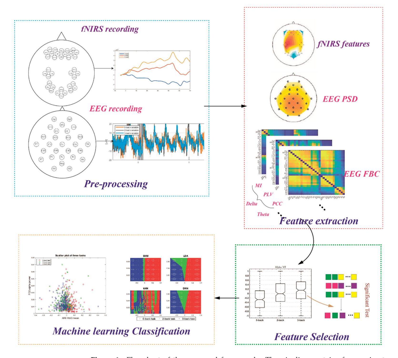
**Figure 1.** Flowchart of the proposed framework. The pipeline contains four main steps: preprocessing, feature extraction, feature selection and machine-learning classification.
39
*Sensors* **2022**, *22*, 7623
#### 2.1. Dataset
This study made use of a dataset gathered by Shin et al. [30] at the Technische Universität Berlin. The dataset comprised scalp recordings—30 EEG channels and 36 fNIRS channels—for mental workload during n-back tasks. The channels and their locations are shown in Supplementary Figure S1. These activities were divided into four categories: 0-, 2-, and 3-back tasks, as well as rest between tasks. Twenty-six healthy, right-handed people took part, and the dataset was divided into three sessions, each with three randomly organized sets of 0-, 2-, and 3-back tasks, meaning that each participant completed nine sets of n-back tasks. A single task consisted ofa2s instruction indicating the type of task (0-, 2-, or 3-back), a 40 s task period that consists of 20 trials, a 1 s stop period, and a 20 s rest period (see Figure 2). Therefore, there were 26 × 3 × 9 = 702 tasks available for all participants. All EEG and fNIRS signals were captured at the same time.
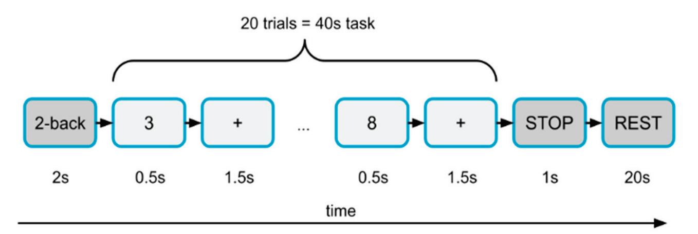
**Figure 2.** Layout of a set in the experiment. A single task consisted of a 2 s instruction indicating the type of task (0-, 2-, or 3-back), a 40 s task period that consisted of 20 trials, a 1 s stop period, and a 20 s rest period. Each participant completed nine sets of n-back tasks.
#### 2.2. Signal Preprocessing and Feature Extraction
#### 2.2.1. fNIRS
fNIRS data were preprocessed using the BBCI toolbox in MATLAB R2019b [31]. The sampling rate was 10 Hz. Initially, HbR and HbO values were calculated using the modified Beer–Lambert equation (mBLL) from the fNIRS optical density [32]. A sample of HbR and HbO values for each participant is shown in Supplementary Figures S2 and S3. Data augmentation was performed to create small informative segments. To reduce noise and artefacts, fNIRS signals were passed through a third-order digital Butterworth filter between 0 and 0.04 Hz. Additionally, baseline correction was applied to the fNIRS signals to remove the intra-individual variance of the starting values. In this step, the segments were normalised by subtracting the median value of the pre-stimulus baseline from the signal in each segment [8].
It should be noted that there was a general 6 s delay between the stimulus representation and peak cortical hemodynamics. This delay was determined by the task and HbR and HbO concentrations. Normally, the cerebral hemodynamic response does not return to baseline until 10 s after stimulus presentation. However, agreement on an ideal time window for analysis had yet to be reached because the best temporal length depended on the paradigm used and participant characteristics, such as age [21]. This paper conducted a sensitivity analysis to identify the optimal time window to produce the most accurate mental workload estimate and a size of 5s was used. The window slides through the whole 40 s period with a 1 s step. This analysis was performed independently for each participant.
#### 2.2.2. EEG
EEG data were also preprocessed using the BBCI toolbox in MATLAB R2019b, and resampling was done at 200 Hz. The improved weight-adjusted second-order blind identification (iWASOBI) method in the automatic artifact removal (AAR) toolbox in EEGLAB was used to gain ocular artifact rejection. Initially, data augmentation was done by segmenting
40
*Sensors* **2022**, *22*, 7623
data samples into smaller but still informative segments. Then, the data were bandpassfiltered between 1 and 45 Hz using a third-order Butterworth digital filter. The EEG epochs were extracted from −500 to 6000 ms with respect to the onset of every stimulus. Power spectral density (PSD) was calculated for three frequency bands of EEG recordings: delta (0.5–4 Hz), theta (4–7 Hz), and alpha (8–15 Hz) since previous studies indicated that lowfrequency information made more contributions for measuring mental workload [7,33]. The FBC was estimated using four methods: Pearson correlation coefficient (PCC), mutual information (MI) in the time domain, magnitude squared coherence (MSC), and phase-locking value (PLV) in the frequency domain. The principal details are given as follows:
The PCC was able to evaluate the linear interdependency between two signals in the time domain and ranged from −1 to +1. The correlation coefficient between signals *x* and *y* were
$$\rho_{xy} = \frac{E\left[\left(x - \mu_x\right)\left(y - \mu_y\right)\right]}{\sigma_x \sigma_y} \tag{1}$$
where *E* is the expected value; *μx* and *μy* are the mean values; and *σx* and *σy* are the standard deviations of the *x* and *y* time series.
MSC is a linear method to estimate interconnections between two signals in the frequency domain calculated by PSD. The MSC of signals *x* and *y* can be written as
$$MSC_{xy}(f) = C_{xy}^{2} = \frac{S_{xy}(f)^{2}}{|S_{xx}(f)| \times |S_{yy}(f)|} (2)$$
where *Sxx*(*f*) and *Syy*(*f*) are the PSDs of signals *x* and *y*, respectively; and *Sxy*(*f*) is the cross PSD at frequency *f* .
According to information theory, the MI of two random variables, *x* and *y*, shows how one is informative for the other one. Let, *P*(*x*) and *P*(*y*) be the probability distributions of random variables *x* and *y*, respectively. The entropy of *x* and *y* is defined as
$$H(x) = -\sum_{j=1}^{N} P(x_j) \log_b(P(x_j))$$
(3)
$$H(y) = -\sum_{j=1}^{N} P(y_j) \log_b(P(y_j))$$
(4)
where *N* defines window length. *H*(*y*|*x*) and *H*(*x*, *y*) represent conditional entropy and joint entropy between *x* and *y*, defined respectively as
$$H(x,y) = -E_x[E_y[\log_b P(x,y)]]$$
(5)
$$H(y|x) = -E_x [ E_y [ \log_b P(y|x) ] ] \tag{6}$$
where *E* is the expected value function. The MI of two random variables *x* and *y* is computed as follows
\(MI(x,y) = H(x) + H(y) - H(x,y) = H(y) - H(y|x)\)
(7)
*MI*(*x*, *y*) = 0 if and only if random variables *X* and *Y* are statistically independent. Notably, the MI is a nonlinear method in the time domain,
Phase synchronisation (PS) assumes that two oscillation systems without amplitude synchronisation can have phase synchronisation. The phase locking value (PLV) is frequently used to obtain the phase synchronisation strength [14]. The instantaneous phase of a signal *X* is given by
$$\varnothing_x(t) = \arctan\frac{\widetilde{x}(t)}{x(t)}$$
(8)
41
*Sensors* **2022**, *22*, 7623
where *x*(*t*) is the Hilbert transform of *x*(*t*) which is defined as
$$\widetilde{x}(t) = \frac{1}{\pi} PV \int_{-\infty}^{+\infty} \frac{x(\tau)}{t - \tau} d\tau \tag{9}$$
where *PV* refers to the Cauchy principal value. The PLV for two signals is defined as
$$PLV = \left| \frac{1}{N} \sum_{j=0}^{N-1} e^{j(\varnothing_x(j\Delta t) - \varnothing_y(j\Delta t))} \right|$$
(10)
where Δ*t* defines the sampling period, and *N* indicates the sample number of each signal [34]. The range of PLV was from 0 to 1, where 0 showed a lack of synchronisation and 1 indicated strict phase synchronisation. Notably, the PLV is a nonlinear method in the frequency domain.
#### 2.3. Feature Selection and Fusion
A large number of features were extracted from EEG and fNIRS. To be more specific, considering three frequency bands (delta, theta and alpha), 28 channels and four FBC methods, there were 3 × 28 = 84 PSD features and 3 × 28 × (28−1)/2 × 4 = 4536 FBC features estimated from the EEG recording. According to the time window analysis of the fNIRS signals, the top-10 best time windows were chosen. Considering the number of channels, there were 10 × 36 = 360 features for fNIRS. The next step was to feed the extracted features into machine learning classifiers to classify three workloads/tasks. To avoid the overfitting problem of machine learning and compare the combined methods fairly with the methods using a single type of feature, a statistical significance test is used to reduce the feature number. One-way analysis of variance (ANOVA) was used to evaluate the significance of differences in the 0-back vs. 2-back vs. 3-back features. The *p*-value was the criterion for selecting the significant features. As a result, the top-10 features with the smallest *p*-values were individually selected from EEG-based and fNIRSbased techniques as classifier input. Furthermore, the top-5 features from EEG (univariate features only) and fNIRS, respectively, were combined, resulting in 10 hybrid features for comparison purposes.
#### 2.4. Machine-Learning Classification
The SVM was applied to achieve workload classification. It constructed an optimal separating hyperplane in the feature space based on the structural risk minimization principle. The selected features extracted from EEG and fNIRS were fed into the SVM with a radial basis function (RBF) kernel. Different machine-learning algorithms were tested and compared, such as the k-nearest neighbour (KNN), decision tree and LDA. The SVM outperformed other methods in classification. Hence, this paper mainly used the SVM with RBF to represent classification results. To avoid overfitting =in the case of limited data, a five-fold cross-validation technique was employed. To be more specific, the dataset of each condition was divided into five subsets, and then five iterations were undertaken to ensure each subset was used for training and testing [15]. That is to say, for each iteration, 80% of the dataset was used for training and the remaining 20% for testing. Consequently, the classification result was calculated by averaging the accuracies from 5 iterations. Totally, there were 3 workload levels × 3 series × 3 sessions × 26 participants = 702 samples. Before being fed into the classifier, the features were normalised from −1 to 1 for each participant to reduce the influence of individual differences.
#### 3. Results
#### 3.1. Time Interval Selection
The selection of the time interval relied on the classification performance implemented on each participant. Figure 3A represents the mean classification accuracy for all participants using fNIRS-based features against the moving time window, and sustained growth
42
*Sensors* **2022**, *22*, 7623
was observed during the first 30 s. After a 25 s oscillation, the accuracy reached its peak when the 45–50 s time window was used. Consequently, the 10 time-windows in the range of 45 to 54 s were selected for the next step of feature extraction. Figure 3B illustrates the changes in classification accuracy against the length of the time window of fNIRS and EEG. Notably, the accuracy of using fNIRS-based features decreased along with the window-size increment for all three classification groups. However, the EEG-based method performed better following the window-size increment and peaks at 40 s, particularly for 0-back vs. 2-back and 0-back vs. 3-back. As a result, the final window-size selections for fNIRS and EEG were 5 and 40 s, respectively. Furthermore, it indicated that the fused features outperformed features from a single modality.
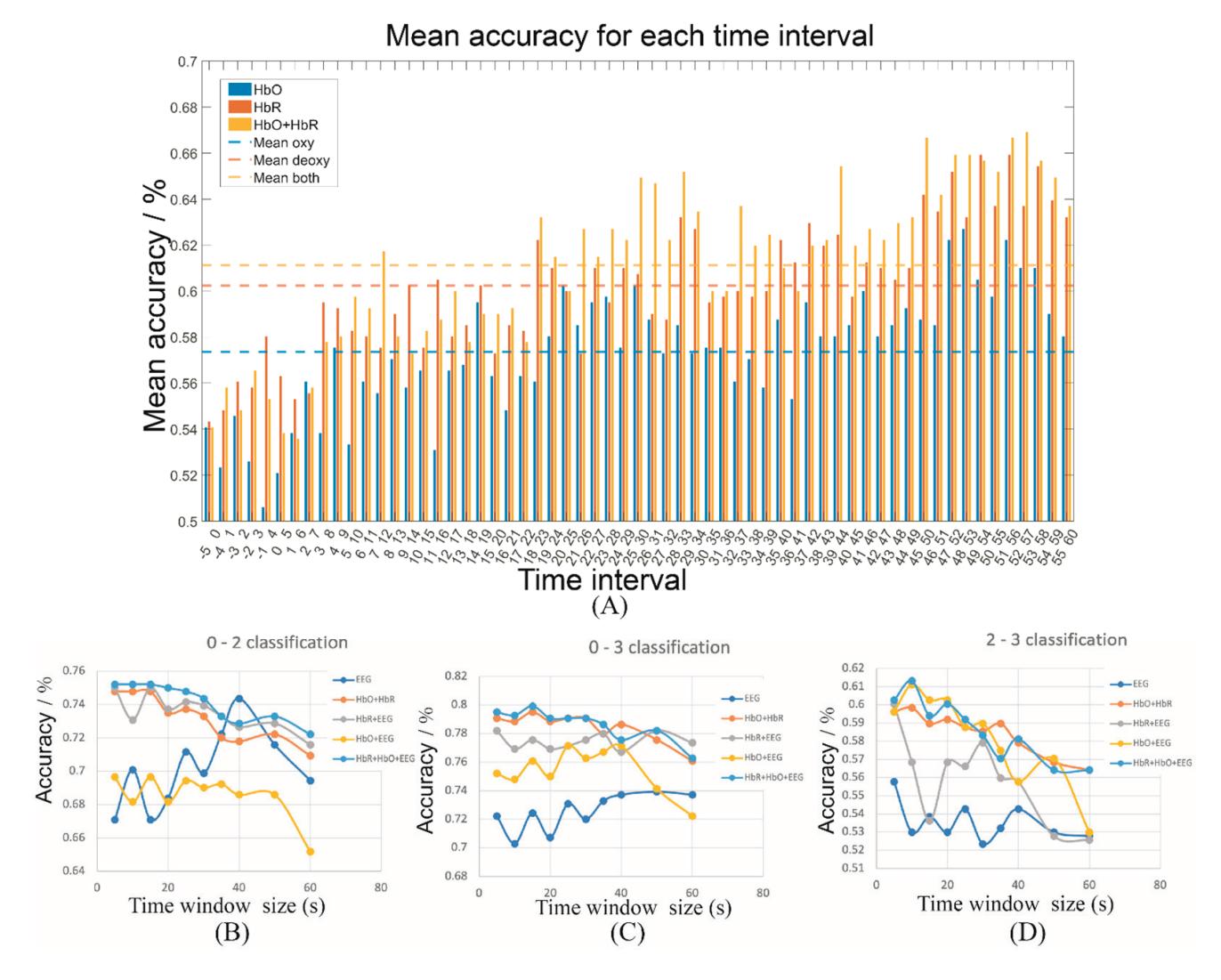
**Figure 3.** Time window analysis (**A**) Time interval analysis for fNIRS features; Time window-size evaluation for EEG and fNIRS features for (**B**) 0-back vs. 2-back, (**C**) 0-back vs. 3-back, (**D**) 2-back vs. 3-back.
#### 3.2. Machine-Learning Classification Performance
To select the optimal FBC features, four different methods (MI, PCC, MSC and PLV) were tested individually, and the nonlinear time-domain method, MI, was found to provide the highest classification accuracy. Figure 4 shows the comparison of the four estimations in the three bands for top-10 average classification accuracy. The error bar shows the accuracy from each iteration of cross-validation. Therefore, MI was selected as the EEG-based FBC feature for the following analysis.
To classify multi-level mental workload, the classification task was separated into three groups: 0-back vs. 2-back, 0-back vs. 3-back and 2-back vs. 3-back. The performances using EEG-based features only, fNIRS-based features only, and hybrid features were evaluated and shown in Tables 2–4. To ensure classification fairness, each classification task used 10 features as the input. The features were selected according to the significance test and a sample is given in Supplementary Figure S4. The EEG alpha band information had the best performance in discriminating the three workload levels for both univariate (PSD) and bivariate features (FBC). Meanwhile, the results also suggested that the FBC features 43
*Sensors* **2022**, *22*, 7623
performed better with an approximately 5% accuracy increment for all three sub-tasks. When it came to fNIRS, HbR outperformed HbO, but the accuracies were both significantly lower than for EEG-based FBC features, particularly for 0-back vs. 2-back and 0-back vs. 3-back. Other references suggested that classifiers, such as LDA, SVM and CNN, achieved higher accuracy using HbR indicators [18,19].
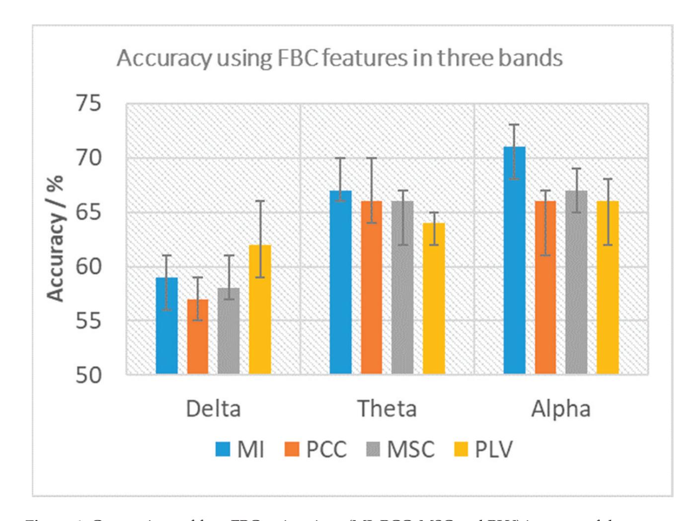
**Figure 4.** Comparison of four FBC estimations (MI, PCC, MSC and PLV) in terms of the average of the Top 10 classification accuracies along with maximum and minimum value.
**Table 2.** SVM classification accuracy of 0-back vs. 2-back using different features.
| | | EEG | | fNIRS | | EEG + fNIRS |
|----------------------|-------|-----|-----|-------|-----|-------------|
| | | PSD | FBC | HbO | HbR | |
| 0-back vs.
2-back | Delta | 66% | 67% | 62% | 68% | 72% |
| | Theta | 68% | 73% | 75% | | |
| | Alpha | 70% | 74% | 77% | | |
**Table 3.** SVM classification accuracy of 0-back vs. 3-back using different features.
| | | EEG | | fNIRS | | EEG + fNIRS |
|----------------------|-------|-----|-----|-------|-----|-------------|
| | | PSD | FBC | HBO | HBR | |
| 0-back vs.
3-back | Delta | 65% | 63% | 62% | 72% | 74% |
| | Theta | 69% | 72% | | | 75% |
| | Alpha | 71% | 77% | | | 83% |
44
*Sensors* **2022**, *22*, 7623
**EEG fNIRS EEG + fNIRS PSD FBC HBO HBR** Delta 52% 60% 57%
Theta 56% 61% 58% Alpha 55% **62%** 59%
**Table 4.** SVM classification accuracy of 2-back vs. 3-back using different features.
Overall, the fused features (EEG–fNIRS) improved classification performance. For the 0-back vs. 2-back and 0-back vs. 3-back tasks, the hybrid method obtains the highest accuracy with 77% (Table 2) and 83% (Table 3), which suggests, as expected, there is more difference between 0-back and 3-back than between 0-back and 2-back. However, the difference between 2-back and 3-back was small, as evident by a much lower accuracy. Notably, the results suggested that the hybrid features did not have superiority in all tasks. As shown in Table 4, the FBC features in the alpha band had the best performance (62%) but the fused features had only 59%. Nevertheless, 2-back and 3-back were difficult to distinguish for any features.
To further evaluate the machine learning algorithms performance, accuracy (*Accu*), sensitivity (*Sens*) and specificity (*Spec*) were calculated:
$$Accu = \frac{TP + TN}{TP + TN + FP + FN} \times 100\% \tag{11}$$
60% 61%
$$Sens = \frac{TP}{TP + FN} \times 100\% \tag{12}$$
$$Spec = \frac{TN}{TN + FP} \times 100\% \tag{13}$$
where *TP* = True Positive; *FN* = False Negative; *TN* = True Negative; and *FP* = False Positive. Moreover, the receiver operating characteristic (ROC) curve, and the area under the ROC curve (AUC) [35,36] were used to assess the goodness of classification. Specifically, the ROC was constructed from the true positive rate (TPR = sensitivity) in the vertical axis and the false positive rate (FPR = 1-specificity) in the horizontal axis [37]. The resulting accuracy, sensitivity, specificity and AUC are shown in Table 5. The ROC curves for three binary classification tasks is shown in Figure 5.
**Table 5.** Performance of classification for 3 binary classification tasks.
| Alpha Hybrid Features | Accuracy | Specificity | Sensitivity | AUC |
|-----------------------|----------|-------------|-------------|--------|
| 0-back vs. 2-back | 77% | 79% | 76% | 0.8332 |
| 0-back vs. 3-back | 83% | 84% | 80% | 0.9501 |
| 2-back vs. 3-back | 59% | 57% | 63% | 0.6721 |
#### 3.3. Visualisation
**2-back vs. 3-back**
To further explore the difference among the three workload levels, a distinct visualisation method was employed. A topographic map was used to represent the PSD distribution of the EEG alpha-band (Figure 6), which provided about 70% classification accuracy for the 0-back vs. 2-back and 0-back vs. 3-back tasks. The averaged PSD distribution across all participants, illustrated by the left column, suggested that the posterior area of 0-back had much higher PSD than 2-back and 3-back, while other areas had similar PSD distribution. It seemed that, during the low workload level, there was more brain activity in the alpha band in the posterior area than during high workload. It matched the classification result, which revealed that the posterior midline occipital (POz), left occipital (O1) and right occipital (O2) channels contributed more than the others. The patterns of 2-back and 3-back are very similar for the whole bran, which explains the low classification accuracy (55%) in Table 4. 45
*Sensors* **2022**, *22*, 7623
The individual PSD distribution, illustrated in the middle column of Figure 6, indicates the difficulty of the classification to an extent. Furthermore, to validate the observation, the right column of Figure 6 shows the accuracy of using each channel's PSD as the input. As expected, the posterior area can provide more than 70% accuracy for 0-back vs. 2-back and 0-back vs. 3-back tasks.
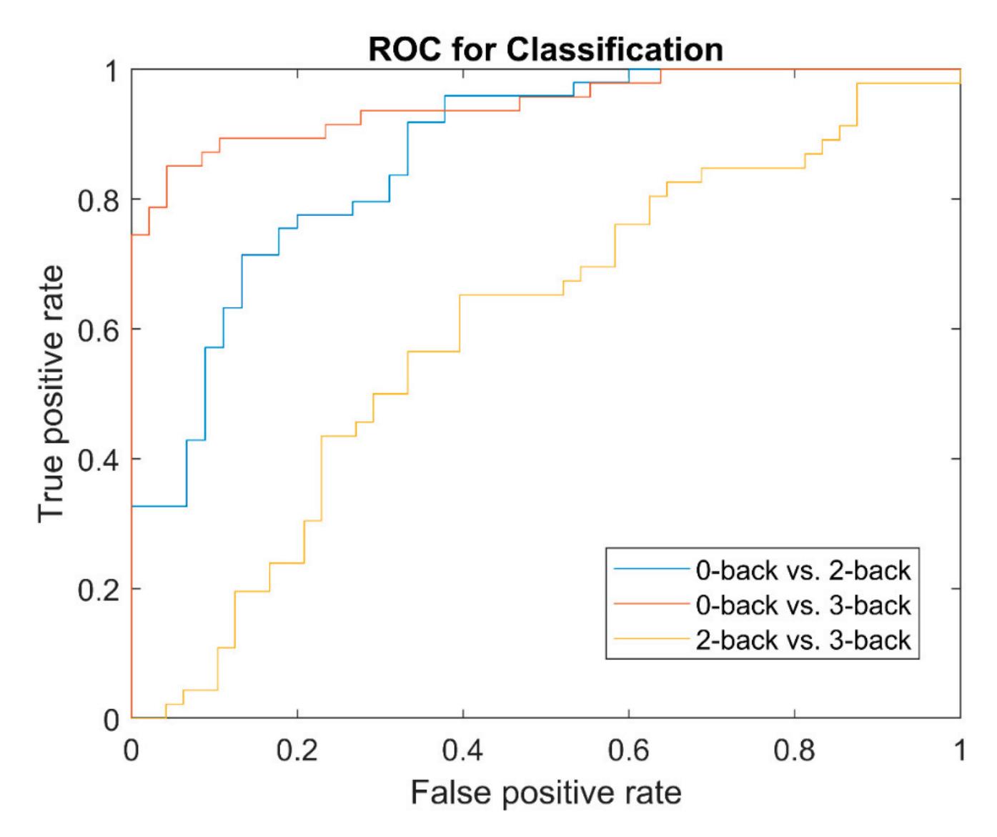
**Figure 5.** The receiver operating characteristic (ROC) curves for three binary classification tasks: 0-back vs. 2-back, 0-back vs. 3-back, and 2-back vs. 3-back.
The topographic map of HbR features is shown in Figure 7**.** Similar to EEG, the averaged HbR distribution of 0-back is significantly different from that of 2-back and 3-back, shown in the left column. More specifically, the frontal-right area has increased HbR following the increment of workload level while the frontal-centre and middle-left areas have decreased HbR following the increment of workload level. All these findings have been supported by the classification result of individual channels (Figure 7). There is no significant difference between 2-back and 3-back in terms of the overall pattern. The individual HbR distribution is illustrated in the middle column of Figure 7. Furthermore, to validate the observation, the right column of Figure 7 shows the accuracy of using each channel's HbR as the input. It is noted that the right frontal area can provide more than 70% accuracy for the 0-back vs. 3-back task. Interestingly, the accuracy of the posterior area (PPOz) was close to 70% for 0-back vs. 2-back and 0-back vs. 3-back tasks, which was not easy to observe from the feature visualisation. It also matched the findings in the EEG analysis.
46
*Sensors* **2022**, *22*, 7623
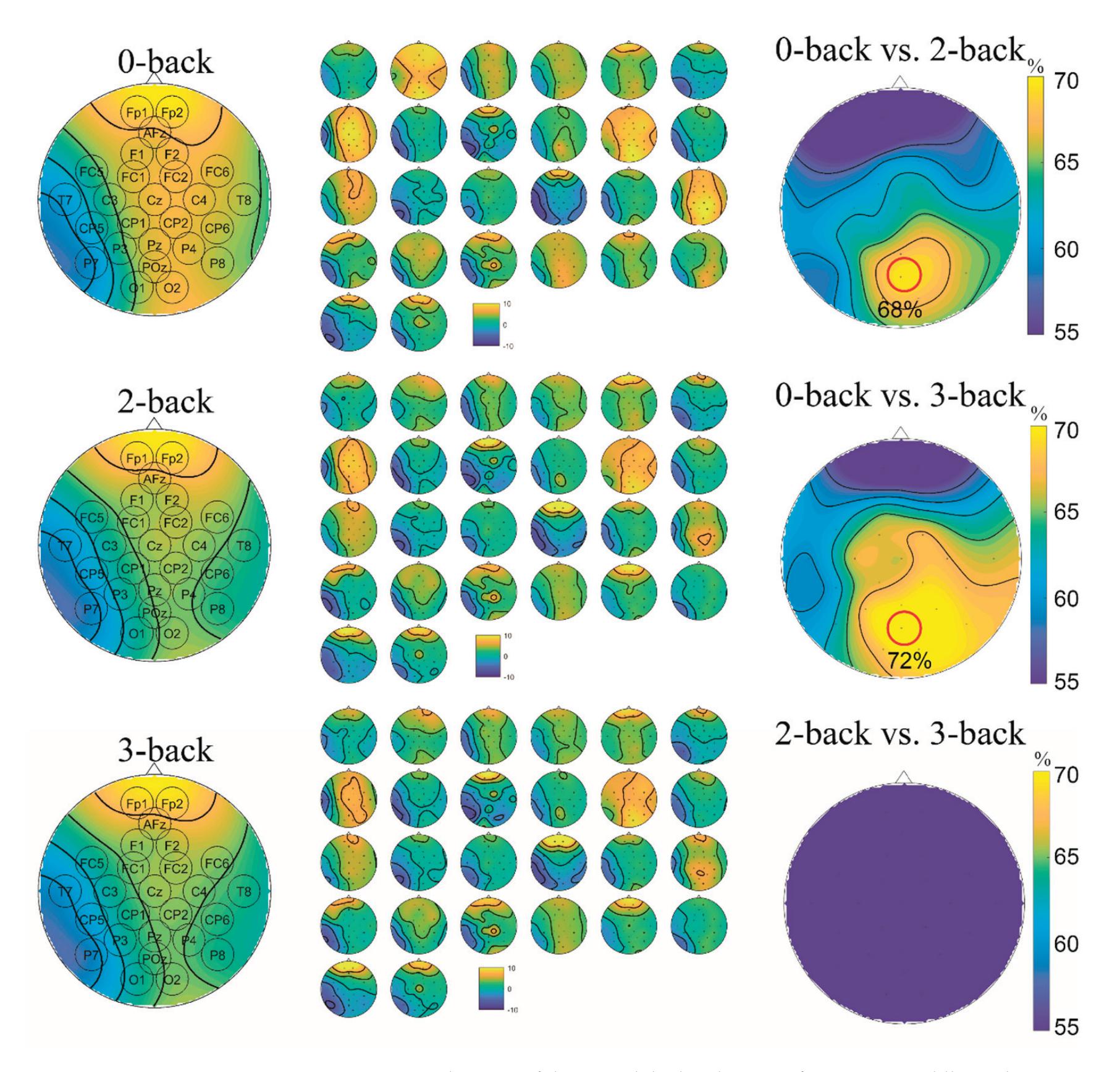
**Figure 6.** Topographic map of the EEG alpha-band PSD. Left: average; Middle: each participant; Right: Accuracy using each-channel PSD as the input. The area that provides the highest accuracy is highlighted.
To visualise the FBC features, a heat map was used as shown in Figure 8. The maps for individual participants are illustrated in Figure 8A–C for 0-back, 2-back and 3-back respectively. The accuracy of the three classification tasks is illustrated in Figure 8D–F for 0-back vs. 2-back, 0-back vs. 3-back, and 2-back vs. 3-back, respectively. It shows that each participant had a similar FBC pattern estimated by MI, while the value of different regions varied. Furthermore, it helped us to understand the differential contribution of the various brain regions for mental workload discrimination. The functional brain connectivity between frontal channels and Fp1 estimated by MI had a significant increase when the workload level became higher. It was also proved in Figure 8D–F that the following pairs left frontopolar–anterior midline frontal (Fp1:AFz), left frontopolar–left frontal (Fp1:F1), left frontopolar–right frontopolar (Fp1:Fp2) and left frontopolar–right frontal (Fp1:F2) provided relatively higher classification accuracy when differentiating 0-back from 2-back and 3-back.
47
*Sensors* **2022**, *22*, 7623
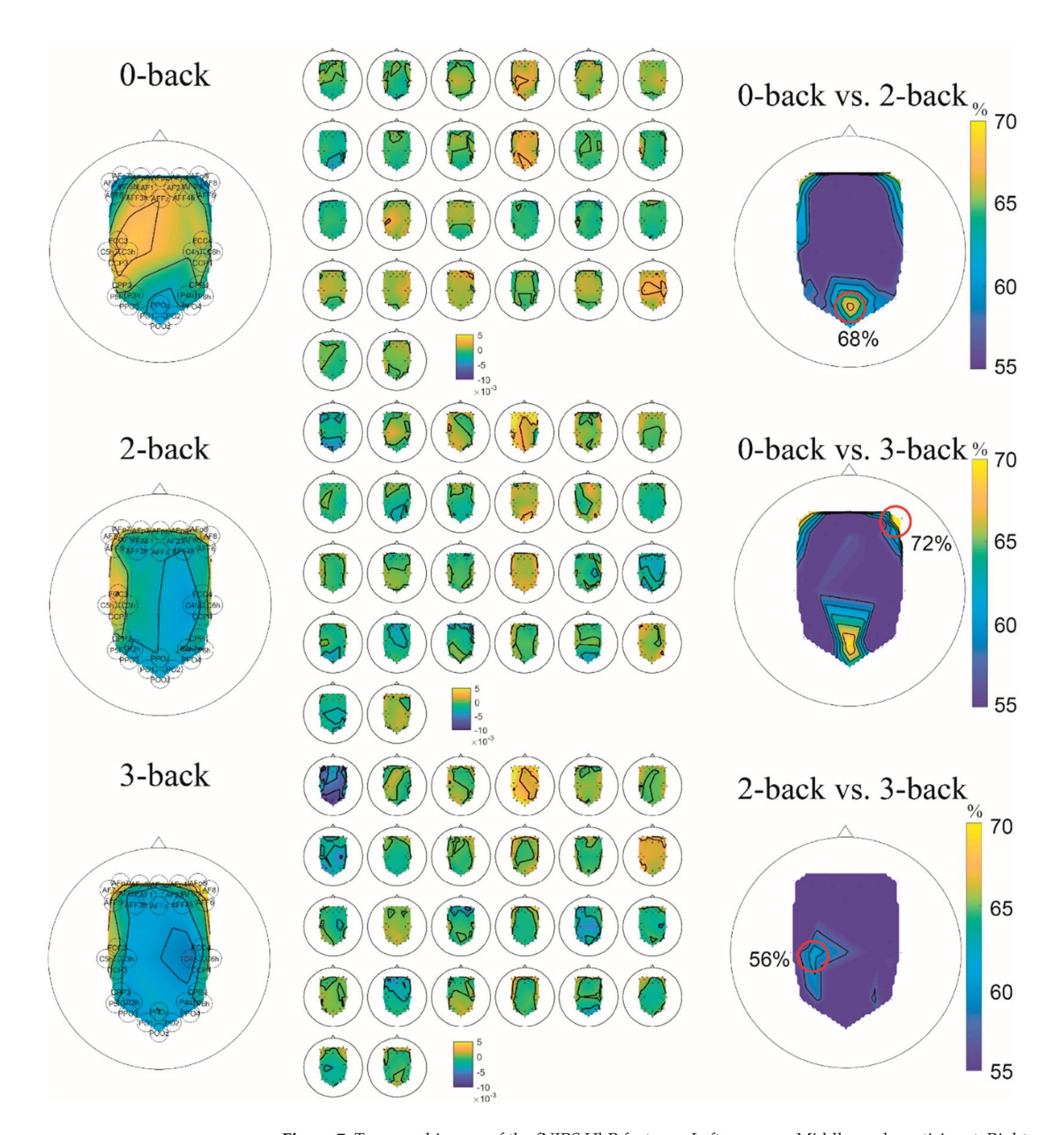
**Figure 7.** Topographic map of the fNIRS HbR features. Left: average; Middle: each participant; Right: Accuracy using each-channel HbR feature as the input. The area that provided the highest accuracy is highlighted.
48
*Sensors* **2022**, *22*, 7623
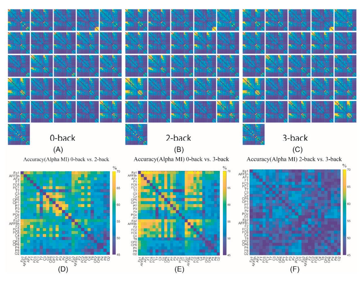
**Figure 8.** The heat map of MI FBC features and the accuracy results. (**A**–**C**) shows the MI value for each participant in 0-back, 2-back, and 3-back task. (**D**–**F**) represents the classification accuracy for 0-back vs. 2-back, 0-back vs.3-back and 2-back vs. 3-back, respectively, using each pair of EEG channels as the input where the FBC value was estimated by MI.
#### 4. Discussion
A comparative analysis of previous research and the proposed work employing EEG and fNIRS in mental workload classification is shown in Table 6. This paper now discusses the results in detail from three aspects: EEG vs. fNIRS, univariate vs. multivariate features, and independent vs. hybrid feature.
**Table 6.** A comparative analysis of the previous research and the proposed work.
| Reference | Study Setting | Classifier | Accuracy |
|----------------------|-----------------------------------------------------|-------------|--------------------------------------------------------------------------------------|
| Liu et al. [28] | 0-, 1-, 2- N-back | LDA | 64.4% (EEG)
55.6% (fNIRS)
68.1% (EEG+fNIRS) |
| Aghajani et al. [10] | 0-, 1-, 2-, 3- N-back | SVM | 85.9% (EEG)
74.8% (fNIRS)
90.9% (EEG+fNIRS) |
| Nguyen et al. [38] | Simulated driving
system | FLDA | 73.7% (EEG)
70.5% (fNIRS)
79.2% (EEG+fNIRS) |
| Saadati et al. [29] | N-back
DSR
Word generation
LHand vs. RHand | DNN, SVM | 67.0% (EEG-DNN)
80.0% (fNIRS-DNN)
87.0% (EEG+fNIRS-DNN)
82% (EEG+fNIRS-SVM) |
| Chu et al. [39] | Mental workload | SVM, RF, DT | 55.4% (EEG-RF)
69.2% (fNIRS-RF)
78.3% (EEG+fNIRS-RF) |
| Proposed study | 0-, 2-, 3-back | SVM | 77% (0-back vs. 2-back)
83% (0-back vs. 3-back)
59% (2-back vs. 3-back) |
Abbreviations: LDA—Linear discriminant analysis; SVM—Support Vector Machine; FLDA—Fisher Linear Discriminant Analysis; DNN—Deep Neural Network; RF—Random Forest; DT—Decision Tree; DSR—discrimination/selection response task.
49
*Sensors* **2022**, *22*, 7623
#### 4.1. EEG vs. fNIRS
On one hand, EEG needed a longer data length to suggest difference between differentlevel workloads. To be more specific, a 40 s time window was the most suitable, while 5 s was suggested for fNIRS. That is to say, fNIRS required less response time to support a satisfactory classification accuracy, which meant it may be more efficient in actual application. On the other hand, the EEG-based features, especially the FBC, represented obvious advantages over the fNIRS-based features in classification accuracy although the FBC methods were more complicated and entailed a higher computational cost.
The best region for assisting in the discrimination of the mental workload was different for EEG and fNIRS. Specifically, the posterior area performed the best for EEG (POz) in the alpha band and fNIRS had superiority in the right frontal region (AF8). Some studies suggested similar findings. Brouwer et al. [33] found the alpha power of the midline parietal (Pz) region in EEG recordings significantly decreased with memory load, effectively distinguishing 2-back from 0-back. Chu et al. [39] stated that the alpha-power of O1 indicated differences between multi-level workloads. Regarding fNIRS, the prefrontal areas were well-accepted for measuring variations in mental workload [40–42]. However, there was limited research pointing out a determined channel that contributes the most. Our study narrowed down the region (right frontal) to support the discrimination of workloads, as evidenced by the topographic visualisation of the machine-learning classification results.
#### 4.2. Univariate vs. Multivariate Features
Considering the EEG features, the bivariate FBC approaches obtained more satisfactory accuracy compared to the univariate PSD features. The results of this study provide evidence to support the hypothesis that the FBC not only estimated the informational intercommunication of separate brain regions but also tracked distinct changes for different levels of workload. There are other supporting studies for this hypothesis in the literature on workload classification. Pei et al. [43] suggested the fusion of band power and FBC features, which were estimated by PLV and the phase lag index (PLI), enhanced the classification performance of workload identification. The PLI-based FBC was also used by Kakkos et al. [7], and the study implied that using FBC emphasised its ability to serve as a promising indicator for different workload levels. Our framework employed four FBC estimations that illustrated connections with various properties, and MI outperformed PCC, MSC and PLV for the highest classification accuracy. In this case, the proposed framework deepened the use of the FBC technique in the field of mental workload discrimination. Furthermore, it implied that, among different levels of workload, the greatest changes occurred in nonlinear brain connectivity.
#### 4.3. Independent vs. Hybrid Feature
The hybrid features of EEG and fNIRS outperformed the independent category of features in classification results, achieving the highest accuracy of 77% for 0-back against 2-back and 83% for 0-back against 3-back. It meant that different methods explored distinct information and became complementary to each other thereby improving classification performance. The results agreed with the conclusion in the literature [29,38,39,42]. The present paper is an advance on previous studies because it generated new knowledge about regional information by comparing the foci of independent types of features. To an extent, it paved the way to use an EEG–fNIRS hybrid sensor in real-world workload classifications.
#### 5. Conclusions
In this paper, a novel solution relying on hybrid EEG–fNIRS features was proposed to deal with multi-level mental workload classification supported by machine-learning classifiers. To be more specific, the univariate PSD and four bivariate FBC features were extracted from an EEG recording in three frequency bands. With the assistance of HbO and HbR indicators from fNIRS, the fused features improved classification performance. Moreover, topographic and heat-map visualisation indicated distinct regions for EEG and
50
*Sensors* **2022**, *22*, 7623
fNIRS that represented difference among 0-back, 2-back and 3-back. Overall, the FBC technique based on an EEG recording proved its value in mental workload classification, and accuracy improvement emphasised the effectiveness of the hybrid EEG–fNIRS. The one limitation of this study was that there was a volume conduction effect in the EEG dataset, but the high classification accuracy suggested that the functional connectivity was effective for classifying different workloads. One potential future work would be to use bipolar channels rather than unipolar channels or to pre-process the data to mitigate volume conduction.
**Supplementary Materials:** The following supporting information can be downloaded at: https: //www.mdpi.com/article/10.3390/s22197623/s1, Figure S1: Channels and locations for the EEG (Left) and fNIRS (Right) recordings; Figure S2: fNIRS average HbR value of each of 26 participants in three levels of workload; Figure S3: fNIRS average HbO value of each of 26 participants in three levels of workload; Figure S4: A sample of significant test to represent the difference among three-level workload with the purpose of selecting limited numbers of features (*p*-value < 0.0001).
**Author Contributions:** Conceptualization, J.C. and Y.Z.; methodology, J.C., E.M.G. and Y.Z.; software, J.C. and Y.Z.; validation, J.C., E.M.G. and Y.Z.; formal analysis, J.C., E.M.G. and Y.Z.; investigation, E.M.G.; resources, E.M.G.; data curation, J.C. and E.M.G.; writing—original draft preparation, J.C.; writing—review and editing, J.C. and Y.Z.; visualization, J.C. and E.M.G.; supervision, Y.Z.; project administration, Y.Z.; funding acquisition, Y.Z. All authors have read and agreed to the published version of the manuscript.
**Funding:** This research received no external funding.
**Institutional Review Board Statement:** Not applicable.
**Informed Consent Statement:** Not applicable.
**Data Availability Statement:** The data presented in this study are available on request from the corresponding author. The data are not publicly available due to privacy.
**Conflicts of Interest:** The authors declare no conflict of interest.
#### References
- 1. Anderson, E.W.; Potter, K.C.; Matzen, L.E.; Shepherd, J.F.; Preston, G.A.; Silva, C.T. A user study of visualization effectiveness using EEG and cognitive load. *Comput. Graph. Forum* **2011**, *30*, 791–800. [CrossRef]
- 2. Bashivan, P.; Yeasin, M.; Bidelman, G.M. Single trial prediction of normal and excessive cognitive load through EEG feature fusion. In Proceedings of the 2015 IEEE Signal Processing in Medicine and Biology Symposium, Philadelphia, PA, USA, 1 December 2016.
- 3. Zhang, J.; Li, S. A deep learning scheme for mental workload classification based on restricted Boltzmann machines. *Cogn. Technol. Work* **2017**, *19*, 607–631. [CrossRef]
- 4. Hussain, I.; Park, S.J. Quantitative evaluation of task-induced neurological outcome after stroke. *Brain Sci.* **2021**, *11*, 900. [CrossRef]
- 5. Hussain, I.; Hossain, A.; Jany, R.; Bari, A.; Uddin, M.; Raihan, A.; Kamal, M.; Ku, Y.; Kim, J. Quantitative Evaluation of EEG-Biomarkers for Prediction of Sleep Stages. *Sensors* **2022**, *22*, 3079. [CrossRef]
- 6. Hussain, I.; Young, S.; Kim, C.H.; Benjamin, H.C.M.; Park, S.J. Quantifying physiological biomarkers of a microwave brain stimulation device. *Sensors* **2021**, *21*, 1896. [CrossRef] [PubMed] 7. Kakkos, I.; Dimitrakopoulos, G.N.; Sun, Y.; Yuan, J.; Matsopoulos, G.K.; Bezerianos, A.; Sun, Y. EEG Fingerprints of Task-
- Independent Mental Workload Discrimination. *IEEE J. Biomed. Health Inform.* **2021**, *25*, 3824–3833. [CrossRef] 8. Pfeifer, M.D.; Scholkmann, F.; Labruyère, R. Signal processing in functional near-infrared spectroscopy (fNIRS): Methodological
- differences lead to different statistical results. *Front. Hum. Neurosci.* **2018**, *11*, 641. [CrossRef]
- 9. Kuanar, S.; Athitsos, V.; Pradhan, N.; Mishra, A.; Rao, K.R. Cognitive Analysis of Working Memory Load from Eeg, by a Deep Recurrent Neural Network. In Proceedings of the ICASSP, IEEE International Conference on Acoustics, Speech and Signal Processing, Calgary, AB, Canada, 15–20 April 2018; Volume 2018, pp. 2576–2580.
- 10. Aghajani, H.; Garbey, M.; Omurtag, A. Measuring mental workload with EEG+fNIRS. *Front. Hum. Neurosci.* **2017**, *11*, 359. [CrossRef]
- 11. So, W.K.Y.; Wong, S.W.H.; Mak, J.N.; Chan, R.H.M. An evaluation of mental workload with frontal EEG. *PLoS ONE* **2017**, *12*, e0174949. [CrossRef]
- 12. Maimon, N.B.; Molcho, L.; Intrator, N.; Lamy, D. Single-channel EEG features during n-back task correlate with working memory load. *arXiv* **2020**, arXiv:2008.04987.
51
*Sensors* **2022**, *22*, 7623
- 13. Mühl, C.; Jeunet, C.; Lotte, F. EEG-based workload estimation across affective contexts. *Front. Neurosci.* **2014**, *8*, 114. [CrossRef] [PubMed]
- 14. Cao, J.; Zhao, Y.; Shan, X.; Wei, H.; Guo, Y.; Chen, L.; Erkoyuncu, J.A.; Sarrigiannis, P.G. Brain functional and effective connectivity based on electroencephalography recordings: A review. *Hum. Brain Mapp.* **2021**, *43*, 860–879. [CrossRef] [PubMed]
- 15. Cao, J.; Grajcar, K.; Shan, X.; Zhao, Y.; Zou, J.; Chen, L.; Li, Z.; Grunewald, R.; Zis, P.; De Marco, M.; et al. Using interictal seizure-free EEG data to recognise patients with epilepsy based on machine learning of brain functional connectivity. *Biomed. Signal Process. Control* **2021**, *67*, 102554. [CrossRef]
- 16. Shan, X.; Huo, S.; Cao, J.; Yang, L.; Zou, J.; Chen, L.; Li, Z. Tracking non-stationary association of two electroencephalography signals using a Revised Hilbert-Huang Transformation. *IEEE Trans. Neural Syst. Rehabil. Eng. Shan* **2021**, *29*, 841–851. [CrossRef]
- 17. Zhao, Y.; Zhao, Y.; Durongbhan, P.; Chen, L.; Liu, J.; Billings, S.A.; Zis, P.; Unwin, Z.C.; De Marco, M.; Venneri, A.; et al. Imaging of Nonlinear and Dynamic Functional Brain Connectivity Based on EEG Recordings with the Application on the Diagnosis of Alzheimer's Disease. *IEEE Trans. Med. Imaging* **2020**, *39*, 1571–1581. [CrossRef] [PubMed]
- 18. Zaman, S.; Rabiul Islam, S. Classification of FNIRS Using Wigner-ville Distribution and CNN. *Int. J. Image, Graph. Signal Process.* **2021**, *13*, 1–13. [CrossRef]
- 19. Alhudhaif, A. An effective classification framework for brain-computer interface system design based on combining of fNIRS and EEG signals. *PeerJ Comput. Sci.* **2021**, *7*, 1–24. [CrossRef] [PubMed]
- 20. Pinti, P.; Tachtsidis, I.; Hamilton, A.; Hirsch, J.; Aichelburg, C.; Gilbert, S.; Burgess, P.W. The present and future use of functional near-infrared spectroscopy (fNIRS) for cognitive neuroscience. *Ann. N. Y. Acad. Sci.* **2020**, *1464*, 5. [CrossRef] [PubMed]
- 21. Herold, F.; Wiegel, P.; Scholkmann, F.; Müller, N.G. Applications of functional near-infrared spectroscopy (fNIRS) neuroimaging in exercise–cognition science: A systematic, methodology-focused review. *J. Clin. Med.* **2018**, *7*, 466. [CrossRef] [PubMed]
- 22. Herff, C.; Heger, D.; Fortmann, O.; Hennrich, J.; Putze, F.; Schultz, T. Mental workload during n-back task-quantified in the prefrontal cortex using fNIRS. *Front. Hum. Neurosci.* **2014**, *7*, 935. [CrossRef] [PubMed]
- 23. Mandrick, K.; Peysakhovich, V.; Rémy, F.; Lepron, E.; Causse, M. Neural and psychophysiological correlates of human performance under stress and high mental workload. *Biol. Psychol.* **2016**, *121*, 62–73. [CrossRef] [PubMed]
- 24. Saadati, M.; Nelson, J.; Ayaz, H. Mental Workload Classification from Spatial Representation of FNIRS Recordings Using Convolutional Neural Networks. In Proceedings of the IEEE International Workshop on Machine Learning for Signal Processing, Pittsburgh, PA, USA, 13–16 October 2019.
- 25. Lim, L.G.; Ung, W.C.; Chan, Y.L.; Lu, C.K.; Sutoko, S.; Funane, T.; Kiguchi, M.; Tang, T.B. A unified analytical framework with multiple fNIRS features for mental workload assessment in the prefrontal cortex. *IEEE Trans. Neural Syst. Rehabil. Eng.* **2020**, *28*, 2367–2376. [CrossRef] [PubMed]
- 26. Putze, F.; Herff, C.; Tremmel, C.; Schultz, T.; Krusienski, D.J. Decoding Mental Workload in Virtual Environments: A fNIRS Study using an Immersive n-back Task. In Proceedings of the Annual International Conference of the IEEE Engineering in Medicine and Biology Society, Berlin, Germany, 23–27 July 2019; pp. 3103–3106.
- 27. Asgher, U.; Ahmad, R.; Naseer, N.; Ayaz, Y.; Khan, M.J.; Amjad, M.K. Assessment and Classification of Mental Workload in the Prefrontal Cortex (PFC) Using Fixed-Value Modified Beer-Lambert Law. *IEEE Access* **2019**, *7*, 143250–143262. [CrossRef]
- 28. Liu, Y.; Ayaz, H.; Shewokis, P.A. Mental workload classification with concurrent electroencephalography and functional nearinfrared spectroscopy. *Brain-Comput. Interfaces* **2016**, *4*, 175–185. [CrossRef]
- 29. Saadati, M.; Nelson, J.; Ayaz, H. Multimodal fNIRS-EEG classification using deep learning algorithms for brain-computer interfaces purposes. *Adv. Intell. Syst. Comput.* **2020**, *953*, 209–220.
- 30. Shin, J.; Von Lühmann, A.; Kim, D.-W.; Mehnert, J.; Hwang, H.-J.; Müller, K.-R. Simultaneous acquisition of EEG and NIRS during cognitive tasks for an open access dataset. *Sci. Data* **2018**, *5*, 1–16. [CrossRef]
- 31. Blankertz, B.; Tangermann, M.; Vidaurre, C.; Fazli, S.; Sannelli, C.; Haufe, S.; Maeder, C.; Ramsey, L.E.; Sturm, I.; Curio, G.; et al. The Berlin brain–computer interface: Non-medical uses of BCI technology. *Front. Neurosci.* **2010**, *4*, 198. [CrossRef]
- 32. Khan, M.J.; Hong, M.J.; Hong, K.-S. Decoding of four movement directions using hybrid NIRS-EEG brain-computer interface. *Front. Hum. Neurosci.* **2014**, *8*, 244. [CrossRef] [PubMed]
- 33. Brouwer, A.M.; Hogervorst, M.A.; Van Erp, J.B.F.; Heffelaar, T.; Zimmerman, P.H.; Oostenveld, R. Estimating workload using EEG spectral power and ERPs in the n-back task. *J. Neural Eng.* **2012**, *9*, 045008. [CrossRef]
- 34. Mormann, F.; Lehnertz, K.; David, P.; Elger, C.E. Mean phase coherence as a measure for phase synchronization and its application to the EEG of epilepsy patients. *Phys. D Nonlinear Phenom.* **2000**, *144*, 358–369. [CrossRef]
- 35. Lotte, F.; Bougrain, L.; Cichocki, A.; Clerc, M.; Congedo, M.; Rakotomamonjy, A.; Yger, F. A review of classification algorithms for EEG-based brain-computer interfaces: A 10 year update. *J. Neural Eng.* **2018**, *15*, 031005. [CrossRef] [PubMed]
- 36. Pyrzowski, J.; Sieminski, M.; Sarnowska, A.; Jedrzejczak, J.; Nyka, W.M. Interval analysis of interictal EEG: Pathology of the alpha rhythm in focal epilepsy. *Sci. Rep.* **2015**, *5*, 16230. [CrossRef] [PubMed]
- 37. Blinowska, K.J.; Rakowski, F.; Kaminski, M.; De Vico Fallani, F.; Del Percio, C.; Lizio, R.; Babiloni, C. Functional and effective brain connectivity for discrimination between Alzheimer's patients and healthy individuals: A study on resting state EEG rhythms. *Clin. Neurophysiol.* **2017**, *128*, 667–680. [CrossRef]
- 38. Nguyen, T.; Ahn, S.; Jang, H.; Jun, S.C.; Kim, J.G. Utilization of a combined EEG/NIRS system to predict driver drowsiness. *Sci. Rep.* **2017**, *7*, 43933. [CrossRef]
52
*Sensors* **2022**, *22*, 7623
- 39. Chu, H.; Cao, Y.; Jiang, J.; Yang, J.; Huang, M.; Li, Q.; Jiang, C.; Jiao, X. Optimized EEG-fNIRS Based Mental Workload Detection Method for Practical Applications. 2021. Available online: https://assets.researchsquare.com/files/rs-683529/v1\_covered.pdf? c=1631874746 (accessed on 30 August 2022).
- 40. Han, W.; Gao, L.; Wu, J.; Pelowski, M.; Liu, T. Assessing the brain 'on the line': An ecologically-valid assessment of the impact of repetitive assembly line work on hemodynamic response and fine motor control using fNIRS. *Brain Cogn.* **2019**, *136*, 103613. [CrossRef] [PubMed]
- 41. Midha, S.; Maior, H.A.; Wilson, M.L.; Sharples, S. Measuring Mental Workload Variations in Office Work Tasks using fNIRS. *Int. J. Hum. Comput. Stud.* **2021**, *147*, 102580. [CrossRef]
- 42. Karran, A.J.; Demazure, T.; Leger, P.M.; Labonte-LeMoyne, E.; Senecal, S.; Fredette, M.; Babin, G. Toward a Hybrid Passive BCI for the Modulation of Sustained Attention Using EEG and fNIRS. *Front. Hum. Neurosci.* **2019**, *13*, 393. [CrossRef] [PubMed]
- 43. Pei, Z.; Wang, H.; Bezerianos, A.; Li, J. EEG-Based Multiclass Workload Identification Using Feature Fusion and Selection. *IEEE Trans. Instrum. Meas.* **2021**, *70*, 1–8. [CrossRef]
53


*Article*
### Spatio-Temporal Neural Dynamics of Observing Non-Tool Manipulable Objects and Interactions
**Zhaoxuan Li 1,\* and Keiji Iramina 2**
- 1 Graduate School of Systems Life Sciences, Kyushu University, Fukuoka 8190395, Japan
- 2 Faculty of Information Science and Electrical Engineering, Kyushu University, Fukuoka 8190395, Japan
- **\*** Correspondence: li.zhaoxuan.631@s.kyushu-u.ac.jp; Tel.: +81-08095204037
**Abstract:** Previous studies have reported that a series of sensory–motor-related cortical areas are affected when a healthy human is presented with images of tools. This phenomenon has been explained as familiar tools launching a memory-retrieval process to provide a basis for using the tools. Consequently, we postulated that this theory may also be applicable if images of tools were replaced with images of daily objects if they are graspable (i.e., manipulable). Therefore, we designed and ran experiments with human volunteers (participants) who were visually presented with images of three different daily objects and recorded their electroencephalography (EEG) synchronously. Additionally, images of these objects being grasped by human hands were presented to the participants. Dynamic functional connectivity between the visual cortex and all the other areas of the brain was estimated to find which of them were influenced by visual stimuli. Next, we compared our results with those of previous studies that investigated brain response when participants looked at tools and concluded that manipulable objects caused similar cerebral activity to tools. We also looked into mu rhythm and found that looking at a manipulable object did not elicit a similar activity to seeing the same object being grasped.
**Keywords:** EEG; functional connectivity; manipulability; object observation; phase locking value
**Citation:** Li, Z.; Iramina, K. Spatio-Temporal Neural Dynamics of Observing Non-Tool Manipulable Objects and Interactions. *Sensors* **2022**, *22*, 7771. https://doi.org/ 10.3390/s22207771
Academic Editors: Yifan Zhao, Yuzhu Guo and Fei He
Received: 4 September 2022 Accepted: 10 October 2022 Published: 13 October 2022
**Publisher's Note:** MDPI stays neutral with regard to jurisdictional claims in published maps and institutional affiliations.

**Copyright:** © 2022 by the authors. Licensee MDPI, Basel, Switzerland. This article is an open access article distributed under the terms and conditions of the Creative Commons Attribution (CC BY) license (https:// creativecommons.org/licenses/by/ 4.0/).
#### 1. Introduction
Tools play a special role among the objects that people usually come in contact with in daily life. Neuroscientists have found confirmatory evidence that using tools can lead to a lasting, discernible change on the perception of someone's own body [1]. Furthermore, looking at a tool can also initiate a series of changes in cerebral activity. Many previous studies demonstrated that observing tools resulted in a left hemisphere advantage, while this did not occur with other objects [2–4]. The most popular explanation for the neural mechanism behind this phenomenon is that tools have the property of "manipulability" and their appearance suggests an associated action or movement [5,6]. In other words, it is reasonable to consider that the tool-associated cerebral activity is at least partly caused by the manipulability of the presented tools. However, in past decades, most studies compared tools with other objects—either manipulable or not (such as a chair or plane that could not be grasped by hand). Therefore, we suspected that some daily objects that can usually be grasped with human hands may also help with launching a similar cognitive process because they possess an almost similar manipulability to those of tools.
The first purpose of this study is to verify the aforementioned hypothesis. Moreover, we aimed to explore the relationship between seeing an object alone vs. seeing an object grasped by a hand. Previous studies have reported that seeing others' hand actions causes a similar cerebral activity to executing the same action [7–9]. In another study, it was found that observing tools and watching others use tools share similar cerebral activities [10]. Because we assumed that objects with manipulability would lead to similar neural circuits to that of tools, it is necessary to investigate whether seeing objects alone and seeing other people grasping these objects have similar electrophysiological features.
*Sensors* **2022**, *22*, 7771. https://doi.org/10.3390/s22207771 https://www.mdpi.com/journal/sensors
54
*Sensors* **2022**, *22*, 7771
In this study, we designed a simple experiment with visual presentation tasks and collected electroencephalography (EEG) data from volunteer participants. By analyzing the functional connectivity and time-frequency features, the similarities and differences between seeing objects alone and watching others interacting with these objects is demonstrated. Furthermore, we also discuss possible explanations for any unexpected results.
#### 2. Materials and Methods
#### 2.1. Experiments
**Materials**: Our hypothesis requires that the objects used as the stimuli need to be manipulable but are not tools. Additionally, a previous visual–somatosensory cross-modal study reported that objects from different categories may not lead to the same neural activity. Therefore, we chose only three objects that often appear in daily life, are easy to hold by hand, and do not have immediate associations with each other. Meanwhile, this design allowed us to use the same stimuli a number of times before participants felt tired. When creating the condition of "seeing an object being grasped" (i.e., participants saw an interaction with an object), to control the variables as much as possible, the conception of an interaction was analyzed first. An interaction includes three elements: subject, object, and a solution to draw a relation between them. Therefore, two more kinds of stimuli were added between "object" and "interaction": in our design, we used a normal human hand as a subject; orange, bottle, and smart phone as objects; and hand grasping as the solution, which is one of the most common forms of manipulability in our daily life. Figure 1a shows the images used as visual stimuli in the experiment.
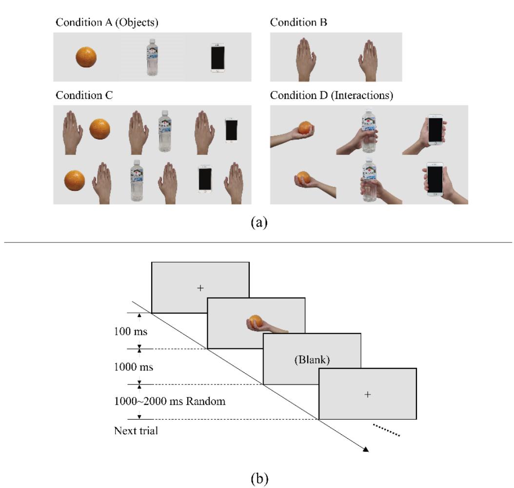
**Figure 1.** (**a**) Four kinds of images used in our experiment. Condition A presented participants with images of an orange, bottle, and smart phone (three objects). Condition B presented images of hands. Condition C combined the three objects and hands within the images. Condition D showed whole actions of hands grabbing objects (interactions). (**b**) Workflow of the trial. The images after the cross were randomly chosen from images corresponding to the current session (e.g., orange session, bottle session, and phone session).
**Participants**: A total of 20 healthy humans (including 8 females; mean age 24.05 years, range 22–27 years) with normal or corrected-to-normal vision participated in this experi55
*Sensors* **2022**, *22*, 7771
ment. This study was reviewed and approved by the Department of Informatics, Faculty of Information Science and Electrical Engineering, Kyushu University (admission No. 2021-13), and every participant signed the informed consent form voluntarily before the experiment began. As all volunteers were right-handed, in this paper, we do not discuss the situation containing the left hand as a stimulus.
**Stimulus presentation**: Visual stimuli were presented to participants on a 17-inch LCD display. The resolution and refresh rate were set at 1280 × 720 pixels and 60 Hz, respectively. The distance between the eyes and display was in the range of 90–100 cm. Two runs were executed for each participant, and each run included three sessions with different topics: orange session, bottle session, and smart phone session. At the beginning of each run, the sequence of the three sessions was decided randomly. In 140 trials for each session, images containing the chosen object (five images from conditions A, C, and D) and subject (two images from condition B) were shown randomly and repetitively (20 times each image) after a fixed cross sign at the center of the screen and then back to a black screen, shown after 1 s, as depicted in Figure 1b. An interval with a duration of 1000–2000 ms was randomly placed between two trials.
#### 2.2. Data Analysis
**EEG data processing**: Data from nineteen participants were included for analyses; data for one were excluded due to an unexpected technical malfunction. The recorded data were re-referenced to a common average, and then sent through a zero-phase-shift frequency domain bandpass filter with the cut-off frequency set at 1 and 30 Hz. Next, the Independent Component Analysis (ICA) completed by the Algorithm for Multiple Unknown Signals Extraction [11] was used to remove EOG artifacts. Trials with potentials over 100 μV were seen as abnormal and abandoned. Finally, over 97.5% of trials of each condition remained for further analysis. The data recorded from 200 ms before stimulus onset (as the baseline) to the end of a trial were extracted as an epoch.
**Statistical test based on Monte Carlo method**: Most of the statistical analysis revealed that the data were not normally distributed; therefore, we chose one-tailed nonparametric test methods for this research. Many researches have proven that the permutation test is reliable for testing neural signals [12,13]. In this research, the workflow can be described as follows:
1. For two independent sample sets, *sampA* and *sampB*, where *H*0 : *sampA* ≤ *sampB*, *v*0 was calculated as follows:
$$v_0 = \overline{sampA} - \overline{sampB}, \tag{1}$$
where *H*0 is the null hypothesis and *v*0 is the test statistic.
2. *sampA* and *sampB* were put into the same group. Then, the elements of this group were randomly divided into two sub-groups: *sampA*1 and *sampB*1, which had the same size. The new statistic of test *v*1 was calculated as follows:
$$v_1 = \overline{sampA_1} - \overline{sampB_1}, \tag{2}$$
- 3. Step b was repeated 10,000 times to obtain *v*1, *v*2, ..., *v*10,000;
- 4. The *v*1, *v*2, ... , *v*10,000 values were sorted in ascending manner, and the sequence number of the first value that was greater than *v*0 was identified as the "*location* ". The *p*-value of the statistic test was calculated as follows:
$$p = 1 - \frac{location}{10,000}$$
Similarly, when it comes to a paired test, we used the bootstrap resampling approach to obtain the confidence interval of the difference between the paired samples. The bootstrap statistical method is also a nonparametric approach with proven validity and has been approved in many studies [14–16]. The procedures are shown below:
56
*Sensors* **2022**, *22*, 7771
1. For two paired sample sets, *sampC* and *sampD*, where *H*0 : *sampC* ≤ *sampD*, we constructed a paired sample set *sampP*, as follows:
$$sampP = sampC - sampD$$
$(4)$
2. Resampling was performed from *sampP* with a replacement to generate a new sample set, *sampP*1; then, its mean value *A*1 was calculated as follows:
$$A_1 = \\\overline{\\text{samp}}P_1$$
(5)
3. The last step was repeated to obtain *A*2, *A*3, ... , *A*10,000, which were then sorted in ascending manner, and then, the index of the first value that was greater than zero was identified as the *index*. The *p*-value of this test was calculated as follows:
$$p' = \frac{index}{10,000'}$$
$(6)$
**Functional connectivity and effective phase-locking value (ePLV)**: We estimated the phase-locking values (PLVs) to measure the connectivity between the data recorded near the occipital lobe (a fusion of EEG recorded from electrodes Oz, O1, O2, POz, PO3, and PO4) and all the other electrodes [17]. The result of the Hilbert Transform (HT) of each epoch was used to generate analytic signals for computing the instantaneous phase at each moment. The PLV between regions *i* and *j* at time *t* is estimated as follows:
$$PLV_{i,j,t} =
\sqrt{\left[\frac{1}{n}\sum_{k=1}^{n}\cos\left(\theta_{i,k,t} - \theta_{j,k,t}\right)\right]^{2} + \left[\frac{1}{n}\sum_{k=1}^{n}\sin\left(\theta_{i,k,t} - \theta_{j,k,t}\right)\right]^{2}}$$
(7)
where *n* is the number of epochs and *θ* is the phase in radians obtained from HT [18]. For each subject, one PLV time series was estimated. However, these values do not always mean that there is a relationship between the two regions because even noise signals would have a PLV between 0 and 1. To know which of them are significantly different from the baseline (effective PLV, ePLV), estimated PLVs were submitted to a bootstrap-resampling-based, paired statistical test program to eliminate false positives by testing with the PLVs during baseline. This program works in two steps: (i) for each participant, the PLVs during the baseline period (i.e., before the stimulus was given) were resampled to extract the mean value according to central-limit theorem, and then (ii) paired tests between PLVs at each moment and the mean value were conducted. The workflow can be described as follows:
For each PLV time series,
- 1. Values during the baseline period were extracted and were put into the baseline vector;
- 2. Resampling was performed from *baseline* with a replacement to obtain a new vector *baseline* with the same size;
- 3. The mean *baseline* across time was calculated;
- 4. Steps 2–3 were repeated 10,000 times and then a grand mean value of the results in step 3 was obtained.
After the above procedures were executed on every PLV time series, a mean value vector was generated as the *baseline*, which was used as a sample set of the control group in the following paired test. Finally, we could determine which of the PLVs represented a meaningful functional connectivity and could be considered as ePLVs.
**Event-related spectral perturbation (ERSP)**: Every epoch was conducted with continuous Morlet wavelet transform to unfold their frequency dimension via the Wavelet Toolbox in MATLAB (MathWorks, Natick, MA, USA). ERSP reflects the energy changes in EEG after providing a stimulus, which is defined as the ratio of power at the current time
57
*Sensors* **2022**, *22*, 7771
and baseline mean [19]. For each epoch, ERSP at time *i* of a specific frequency component *j* can be calculated as follows:
$$ERSP_{i,j} = 10 \times \log_{10} \frac{u_{i,j}}{baseline_j}, \tag{8}$$
where *ui*,*j* is the absolute value of potential at time *i* and frequency *j*, and *baselinej* is the average of the one at frequency *j* before the stimulus was presented. To highlight the source of ERSP variation at the sensor level, a finite difference-based spatial Laplacian transformation was conducted via Brainstorm [20–22]. This procedure used the ERSP data to replace the potential data in the algorithm [23].
#### 3. Results
#### 3.1. Functional Connectivity
It is noticed that functional connectivity estimated by EEG filtered at different bands is totally inconsistent [24]. Therefore, the preprocessed EEG epochs were filtered into four different bands (delta: 1–3 Hz, theta: 4–7 Hz, alpha: 8–13 Hz, and beta: 14–30 Hz); next, the PLVs between EEG recorded at the occipital lobe and other locations were then calculated and the ePLVs were then screened out. The number of ePLVs varied over time. The topography shown in Figure 2 displays the distribution of ePLVs calculated with data from the four frequency bands at different moments. These moments were selected to show as many connections as possible. To highlight the common and different regions that were connected to the occipital lobe, the connections observed when participants saw images of interactions were overlaid on top of those for participants presented with images of objects.
At the delta and alpha bands, the number of ePLVs was fewer than that of the other bands; furthermore, across the three objects, there was a noteworthy change in the moment that the maximum number of connections appeared. By contrast, the ePLVs estimated at the theta band and the beta band were more credible because of the number of observed connections, especially their stability across time and objects.
There were much more functional connections observed when the images from condition D were presented to participants. The results at the theta band suggested a common region including the right frontal lobe (RF), the bilateral central sulcus (L/RCS), and the right angular gyrus (RAG) whenever participants saw objects or interactions. The connection between the occipital lobe and the area covered by electrodes F5, F7, FC5, and FT7 seemed much clearer when seeing interactions than when seeing objects, and so did the left angular gyrus (LAG). Additionally, the moment that a maximum connection number appeared showed a regular pattern: "seeing objects being grasped by human hand" established more connections at earlier. The above results also supported the opinion that the theta band has advantages in observing functional connectivity [25–27].
Beta band ePLVs commonly appeared at both the central frontal lobe (CF) and RAG (near electrode P4 or P6) at the end of a trial, robustly. Meanwhile, the difference between seeing objects and seeing interactions is uncertain; their exclusive regions varied across objects.
In summary, the topography demonstrated that functional connectivity between the occipital lobe and regions of RF, L/RCS, RAG, and CF were established similarly when participants either saw images of objects or those of interactions. To make it more intuitive, the PLV-over-time plot of the regions mentioned above is shown in Figure 3. On the contrary, the difference is embodied in the area covered by electrodes F5, F7, FC5, and FT7, which is believed to be Broca's area (BA) [28–31] and the LAG. Same as before, we demonstrated these differences in the plot of PLV over time in Figure 4. The results of paired test suggested that these differences are significant.
58
*Sensors* **2022**, *22*, 7771
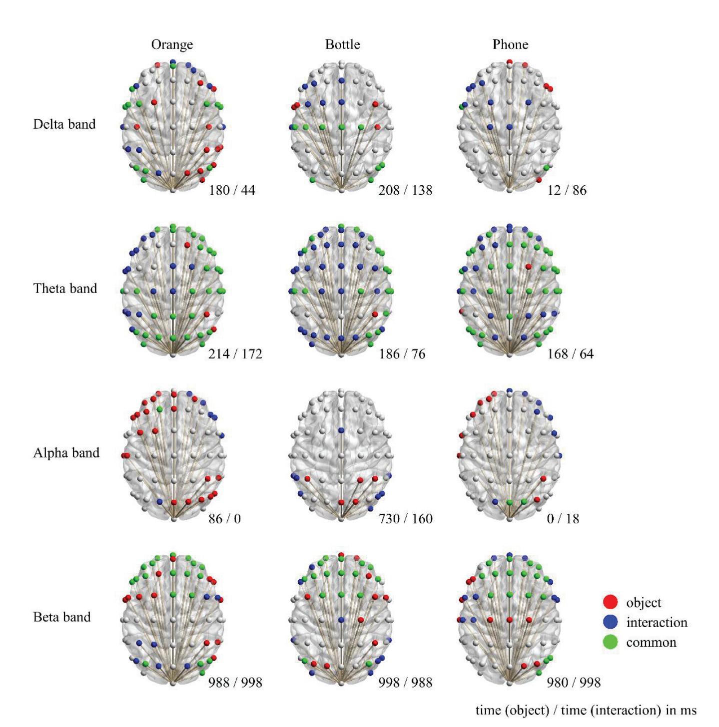
**Figure 2.** Functional connectivity between visual cortex and other regions. Colored electrode indicates that connectivity between that region and the occipital lobe actually exists. Time is indicated at the bottom right corner of each topography, as "time (ms) that most connectivity occurred when seeing objects/time (ms) that most connectivity occurred when seeing objects being grasped". Note that each topography is an overlay of two graphs at two different moments. Red and blue electrodes represent the connections that only occurred when seeing objects and when seeing objects being grasped, respectively, while the green ones mean the two conditions share the same electrode.
#### 3.2. Power Variations
As mentioned in the Introduction, we were expecting to find some motor-related EEG features when participants looked at non-tool objects. Thus, our attention was turned to power changes in the mu rhythm [32–34], and clear event-related desynchronization (ERD) was noticed with both "seeing objects" and "seeing interactions", as shown in Figure 5a. The topography was drawn with EEG data filtered at 8–13 Hz and then was Laplacian spatial filtered to highlight the changes. ERD was mainly observed at the region of the bilateral postcentral gyrus, which may suggest the participation of the primary somatosensory cortex [35]. Among all three objects, the most obvious ERD occurred at the area covered by electrodes C5, CP3, and CP5 in the left hemisphere (LS), as well as the corresponding position in the right hemisphere (RS). Figure 5b revealed its dynamic changes over time. Although all of these plots performed clear ERD at the end, there was obvious event-related synchronization (ERS) observed during the process when participants saw objects being grasped. This ERS was widespread from 100 to 200 ms, especially in LS.
59
*Sensors* **2022**, *22*, 7771
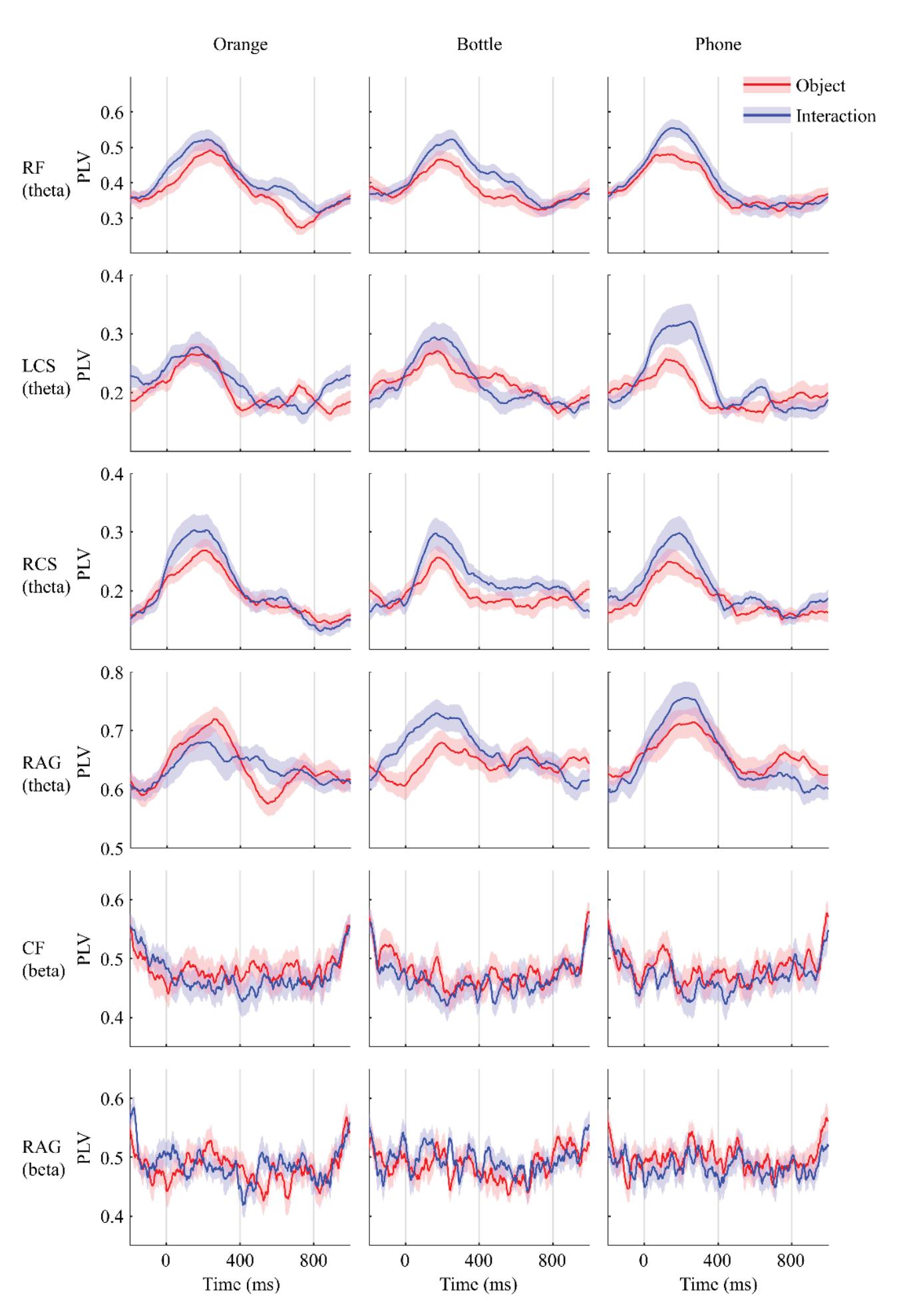
**Figure 3.** PLVs over time. Red line shows phase locking values (PLVs) when participants were shown objects, while the blue line shows PLVs when they were shown objects being grasped by human hands. Shaded areas are standard error. On these shown regions, PLVs from the two conditions varied similarly for the theta and beta bands.
60
*Sensors* **2022**, *22*, 7771
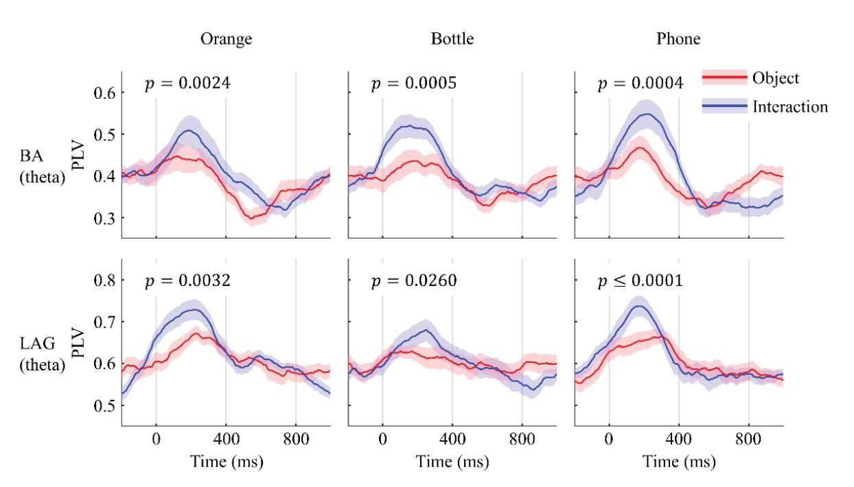
**Figure 4.** PLV observed at BA and LAG. Red line shows PLVs when participants were shown objects, while the blue line shows PLVs when they were shown objects being grasped by human hands. Shaded areas are standard error. Significant difference was noticed between seeing objects and seeing interactions at 200 ms after presenting the stimulus to participants (α = 0.05).
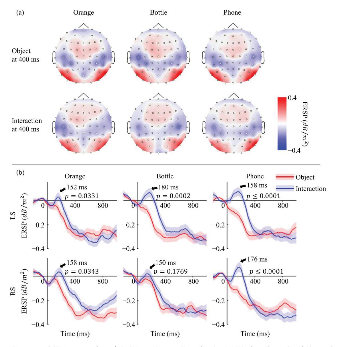
**Figure 5.** (**a**) Topography of ERSP at 400 ms. Mu rhythm ERD distributed at bilateral posterior central gyrus with a little left advantage and performed similarly in all six situations. (**b**) ERSP over time. Red line shows ERSP when participants were shown objects, while the blue line shows ERSP when they were shown objects being grasped by human hands. Shaded areas are standard error. A clear ERS was observed only when seeing interactions, and its peak time is indicated with an arrow. The significance of ERS was confirmed by a permutation test on the ERSP value in the two conditions at the corresponding time (α = 0.05).
61
*Sensors* **2022**, *22*, 7771
#### 4. Discussion
The purpose of this study was to investigate whether seeing manipulable objects would lead to a similar phenomenon to that when seeing tools. A previous research studied the difference between tools and "objects without manipulability" and reported that the stage of confirming whether a presented object is able to be operated happens in the first 250 ms after visual stimulus onset, and the conclusion leads to the activation of the left somatosensory cortex and the bilateral premotor cortex [36]. Moreover, they also mentioned that Brodmann areas 19 and 37 were activated in the ventral side, whether the object was manipulable or not. In our study, we noticed the functional connectivity peaked at 200 ms approximately between the visual cortex and RAG (BA39, border on BA19 and BA37) and between RF (close to the premotor cortex in the right hemisphere) and LCS (the left somatosensory cortex). However, we did not find enough evidence to imply the participation of the left premotor cortex. Additionally, our results indicated that RCS also joined the cognition process after seeing a manipulable object. Another study that paid attention to the mu rhythm ERD phenomenon when seeing tools found that it can be noticed as early as in the first 175 ms [37]. These spatial and temporal commonalities suggested the perception of a manipulable object is similar to those of tools.
Many studies considered that the particularity of tools is derived from the action applied to use them, which they come naturally with [38]. Therefore, we suspected that the presentation of a manipulable object may cause a similar cerebral activity to that which occurs upon seeing an interaction with that object. However, our experimental results rejected this inference with the additional functional connectivity between the occipital lobe and BA as well as between the occipital lobe and LAG when participants were shown images of objects being grasped. Although the controversy about its location is still ongoing, a large majority of scholars believe that the mirror neuro system (MNS) exists near Broca's area (or BA44), the inferior parietal lobule (near the LAG), and the superior temporal sulcus [39–42]. Hence, connectivity observed at BA and LAG can be reasonably regarded as activity of the MNS evoked by seeing the action of grasping objects. This may explain the different distributions of functional connectivity for seeing objects vs. seeing interactions with objects; nevertheless, ERS in the somatosensory cortex, which can only be noticed in the latter case, still exists. All of this evidence led us to the conclusion that the changes observed in the cerebral cortex after seeing objects being grasped were not the same as those that occurred after seeing only objects.
Undoubtedly, the difference in power change in the somatosensory cortex is due to the difference in visual stimuli, which means that the ERS may be caused by the hand contained within the image or the combination of a hand and the object. Fortunately, we have collected EEG data from when participants were shown only a hand and both a hand and an object. By comparing the topography in Figure 6a, we found that they showed ERS in the left somatosensory cortex for both conditions, although the values were not completely the same. This suggests that the hand seen in the visual stimuli partly contributed to the ERS. We also analyzed the data from condition C and interestingly found that it was different from that of the other three kinds of stimulus. It seems that participants recognized the hand and object in each image as two entities. We found that, at about 200 ms after visual stimulus onset, a positive event-related potential (ERP) component appeared at both the PO7 and PO8 electrodes but with a right hemisphere asymmetry. The plot in Figure 6b shows the ERP difference between the PO7 and PO8 electrodes. Evidently, two clear peaks were observed in condition C, while only one was observed in the other two conditions. A further test with a one-way ANOVA-based multiple comparison suggested that the laterization phenomenon in condition C was significantly different from the others (*p* < 0.05).
62
*Sensors* **2022**, *22*, 7771
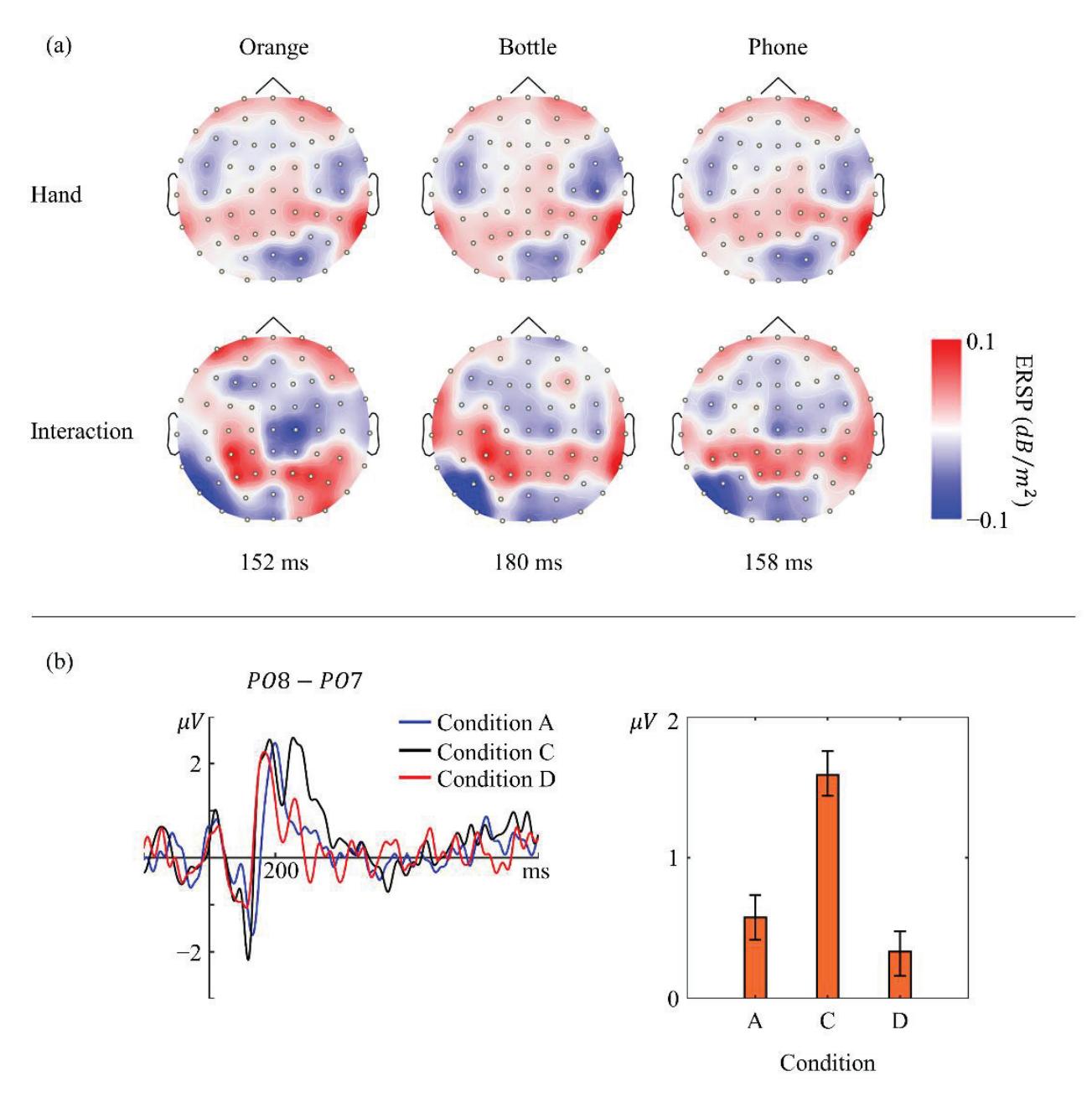
**Figure 6.** (**a**) Topography of 8–13 Hz ERSP when seeing human right hand and seeing interactions using the right hand at 152, 180, and 158 ms. ERS at LS is weaker when only images of a hand are presented to participants. (**b**) Plot shows a grand averaged ERP difference between electrodes PO7 and PO8. A remarkable second peak (black line) appeared when participants were presented with images in condition C. The bar graph on the right shows mean and standard error of the difference data in the range from 246 to 300 ms.
In summary, this study investigated the functional connectivity between the visual cortex and the other regions after healthy participants saw daily objects that are manipulable; we compared our results with those of previous studies regarding brain activity after seeing tools. We found that seeing manipulable objects and seeing tools caused similar phenomena in both time and space. Next, we assessed whether seeing a manipulable object led to a similar mu rhythm change to seeing an interaction with the same object; however, the evidence rejected our hypothesis: additional activation of Broca's area and the left angular gyrus, and early alpha band ERS in the somatosensory cortex were only observed when participants saw interactions.
**Author Contributions:** Conceptualization, Z.L.; methodology, Z.L.; software, Z.L.; validation, K.I.; formal analysis, Z.L.; investigation, Z.L.; resources, Z.L.; data curation, Z.L.; writing—original draft preparation, Z.L.; writing—review and editing, K.I.; visualization, Z.L.; supervision, K.I.; project administration, K.I.; funding acquisition, Z.L. and K.I. All authors have read and agreed to the published version of the manuscript.
**Funding:** This work was supported in part by the JST SPRING, grant Number JPMJSP2136.
63
*Sensors* **2022**, *22*, 7771
**Institutional Review Board Statement:** The study was conducted in accordance with the Declaration of Helsinki and approved by the Institutional Review Board of Kyushu University (protocol code ISEE(ADMITTED)2021-13 and on 30 June 2021).
**Informed Consent Statement:** Informed consent was obtained from all subjects involved in the study.
**Data Availability Statement:** The data presented in this study are available from the corresponding author upon request. The data are not publicly available due to restrictions for participant privacy.
**Acknowledgments:** Thanks to De Bi for being the hand model. Thanks to Yuliang Chen and Yueling Zhang for helping with recruiting volunteers.
**Conflicts of Interest:** The authors declare no conflict of interest.
#### References
- 1. Cardinali, L.; Frassinetti, F.; Brozzoli, C.; Urquizar, C.; Roy, A.C.; Farnè, A. Tool-Use Induces Morphological Updating of the Body Schema. *Curr. Biol.* **2009**, *19*, R478–R479. [CrossRef] [PubMed]
- 2. Verma, A.; Brysbaert, M. A Right Visual Field Advantage for Tool-Recognition in the Visual Half-Field Paradigm. *Neuropsychologia* **2011**, *49*, 2342–2348. [CrossRef] [PubMed]
- 3. Chao, L.L.; Martin, A. Representation of Manipulable Man-Made Objects in the Dorsal Stream. *Neuroimage* **2000**, *12*, 478–484. [CrossRef]
- 4. Garcea, F.E.; Almeida, J.; Mahon, B.Z. A Right Visual Field Advantage for Visual Processing of Manipulable Objects. *Cogn. Affect. Behav. Neurosci.* **2012**, *12*, 813–825. [CrossRef] [PubMed]
- 5. McNair, N.A.; Harris, I.M. Disentangling the Contributions of Grasp and Action Representations in the Recognition of Manipulable Objects. *Exp. Brain Res.* **2012**, *220*, 71–77. [CrossRef] [PubMed]
- 6. Ni, L.; Liu, Y.; Yu, W. The Dominant Role of Functional Action Representation in Object Recognition. *Exp. Brain Res.* **2019**, *237*, 363–375. [CrossRef] [PubMed]
- 7. Marty, B.; Bourguignon, M.; Jousmäki, V.; Wens, V.; de Beeck, M.O.; Van Bogaert, P.; Goldman, S.; Hari, R.; De Tiège, X. Cortical Kinematic Processing of Executed and Observed Goal-Directed Hand Actions. *Neuroimage* **2015**, *119*, 221–228. [CrossRef]
- 8. Buccino, G. Action Observation Treatment: A Novel Tool in Neurorehabilitation. *Philos. Trans. R. Soc. B Biol. Sci.* **2014**, 369. [CrossRef]
- 9. Vogt, S.; Di Rienzo, F.; Collet, C.; Collins, A.; Guillot, A. Multiple Roles of Motor Imagery during Action Observation. *Front. Hum. Neurosci.* **2013**, *7*, 807. [CrossRef]
- 10. Rüther, N.N.; Brown, E.C.; Klepp, A.; Bellebaum, C. Observed Manipulation of Novel Tools Leads to Mu Rhythm Suppression over Sensory-Motor Cortices. Behav. *Brain Res.* **2014**, *261*, 328–335. [CrossRef]
- 11. Tong, L.; Liu, R.-w.; Soon, V.C.; Huang, Y.F. Indeterminacy and Identifiability of Blind Identification. *IEEE Trans. Circuits Syst.* **1991**, *38*, 499–509. [CrossRef]
- 12. Maris, E.; Oostenveld, R. Nonparametric Statistical Testing of EEG- and MEG-Data. *J. Neurosci. Methods* **2007**, *164*, 177–190. [CrossRef] [PubMed]
- 13. Groppe, D.M.; Urbach, T.P.; Kutas, M. Mass Univariate Analysis of Event-Related Brain Potentials/Fields I: A Critical Tutorial Review. *Psychophysiology* **2011**, *48*, 1711–1725. [CrossRef]
- 14. Graimann, B.; Huggins, J.E.; Levine, S.P.; Pfurtscheller, G. Visualization of Significant ERD/ERS Patterns in Multichannel EEG and ECoG Data. *Clin. Neurophysiol.* **2002**, *113*, 43–47. [CrossRef]
- 15. Darvas, F.; Pantazis, D.; Kucukaltun-Yildirim, E.; Leahy, R.M. Mapping Human Brain Function with MEG and EEG: Methods and Validation. *Neuroimage* **2004**, *23*, S289–S299. [CrossRef]
- 16. Delorme, A.; Makeig, S. EEGLAB: An Open Source Toolbox for Analysis of Single-Trial EEG Dynamics Including Independent Component Analysis. *J. Neurosci. Methods* **2004**, *134*, 9–21. [CrossRef]
- 17. Catrambone, V.; Greco, A.; Averta, G.; Bianchi, M.; Valenza, G.; Scilingo, E.P. Predicting Object-Mediated Gestures from Brain Activity: An EEG Study on Gender Differences. *IEEE Trans. Neural Syst. Rehabil. Eng.* **2019**, *27*, 411–418. [CrossRef]
- 18. Lachaux, J.-P.; Rodriguez, E.; Martinerie, J.; Varela, F.J. Measuring Phase Synchrony in Brain Signals. *Hum Brain Mapp.* **1999**, *8*, 194–208. [CrossRef]
- 19. Makeig, S. Auditory Event-Related Dynamics of the EEG Spectrum and Effects of Exposure to Tones. Electroencephalogr. *Clin. Neurophysiol.* **1993**, *86*, 283–293. [CrossRef]
- 20. Pernier, J.; Perrin, F.; Bertrand, O. Scalp Current Density Fields: Concept and Properties. Electroencephalogr. *Clin. Neurophysiol.* **1988**, *69*, 385–389. [CrossRef]
- 21. Nunez, P.L.; Westdorp, A.F. The Surface Laplacian, High Resolution EEG and Controversies. *Brain Topogr.* **1994**, *6*, 221–226. [CrossRef] [PubMed]
- 22. Carvalhaes, C.; De Barros, J.A. The Surface Laplacian Technique in EEG: Theory and Methods. *Int. J. Psychophysiol.* **2015**, *97*, 174–188. [CrossRef]
- 23. Oostenveld, R.; Fries, P.; Maris, E.; Schoffelen, J.M. FieldTrip: Open Source Software for Advanced Analysis of MEG, EEG, and Invasive Electrophysiological Data. *Comput. Intell. Neurosci.* **2011**, 2011. [CrossRef]
64
*Sensors* **2022**, *22*, 7771
- 24. Pockett, S.; Bold, G.E.J.; Freeman, W.J. EEG Synchrony during a Perceptual-Cognitive Task: Widespread Phase Synchrony at All Frequencies. *Clin. Neurophysiol.* **2009**, *120*, 695–708. [CrossRef]
- 25. Sauseng, P.; Klimesch, W.; Schabus, M.; Doppelmayr, M. Fronto-Parietal EEG Coherence in Theta and Upper Alpha Reflect Central Executive Functions of Working Memory. *Int. J. Psychophysiol.* **2005**, *57*, 97–103. [CrossRef]
- 26. Murias, M.; Webb, S.J.; Greenson, J.; Dawson, G. Resting State Cortical Connectivity Reflected in EEG Coherence in Individuals with Autism. *Biol. Psychiatry* **2007**, *62*, 270–273. [CrossRef]
- 27. Fellrath, J.; Mottaz, A.; Schnider, A.; Guggisberg, A.G.; Ptak, R. Theta-Band Functional Connectivity in the Dorsal Fronto-Parietal Network Predicts Goal-Directed Attention. *Neuropsychologia* **2016**, *92*, 20–30. [CrossRef] [PubMed]
- 28. Fadiga, L.; Craighero, L.; D'Ausilio, A. Broca's Area in Language, Action, and Music. *Ann. N. Y. Acad. Sci.* **2009**, *1169*, 448–458. [CrossRef] [PubMed]
- 29. Rizzolatti, G.; Fadiga, L.; Gallese, V.; Fogassi, L. Premotor Cortex and the Recognition of Motor Actions. *Cogn. Brain Res.* **1996**, *3*, 131–141. [CrossRef]
- 30. Fadiga, L.; Craighero, L. Hand Actions and Speech Representation in Broca's Area. *Cortex* **2006**, *42*, 486–490. [CrossRef]
- 31. Fazio, P.; Cantagallo, A.; Craighero, L.; D'ausilio, A.; Roy, A.C.; Pozzo, T.; Calzolari, F.; Granieri, E.; Fadiga, L. Encoding of Human Action in Broca's Area. *Brain* **2009**, *132*, 1980–1988. [CrossRef]
- 32. Jeannerod, M. The Representing Brain: Neural Correlates of Motor Intention and Imagery. *Behav. Brain Sci.* **1994**, *17*, 187–202. [CrossRef]
- 33. Pfurtscheller, G.; Neuper, C. Motor Imagery Activates Primary Sensorimotor Area in Humans. *Neurosci. Lett.* **1997**, *239*, 65–68. [CrossRef]
- 34. Caldara, R.; Deiber, M.P.; Andrey, C.; Michel, C.M.; Thut, G.; Hauert, C.A. Actual and Mental Motor Preparation and Execution: A Spatiotemporal ERP Study. *Exp. Brain Res.* **2004**, *159*, 389–399. [CrossRef]
- 35. Oostenveld, R.; Praamstra, P. The Five Percent Electrode System for High-Resolution EEG and ERP Measurements. *Clin. Neurophysiol.* **2001**, *112*, 713–719. [CrossRef]
- 36. Proverbio, A.M.; Adorni, R.; D'Aniello, G.E. 250 Ms to Code for Action Affordance during Observation of Manipulable Objects. *Neuropsychologia* **2011**, *49*, 2711–2717. [CrossRef]
- 37. Proverbio, A.M. Tool Perception Suppresses 10-12Hz μ Rhythm of EEG over the Somatosensory Area. *Biol. Psychol.* **2012**, *91*, 1–7. [CrossRef]
- 38. Creem-Regehr, S.H.; Lee, J.N. Neural Representations of Graspable Objects: Are Tools Special? Cogn. *Brain Res.* **2005**, *22*, 457–469. [CrossRef] [PubMed]
- 39. Rizzolatti, G.; Craighero, L. The Mirror-Neuron System. *Annu. Rev. Neurosci.* **2004**, *27*, 169–192. [CrossRef]
- 40. Gallese, V.; Fadiga, L.; Fogassi, L.; Rizzolatti, G. Action Recognition in the Premotor Cortex. *Brain* **1996**, *119*, 593–609. [CrossRef]
- 41. Cerri, G.; Cabinio, M.; Blasi, V.; Borroni, P.; Iadanza, A.; Fava, E.; Fornia, L.; Ferpozzi, V.; Riva, M.; Casarotti, A.; et al. The Mirror Neuron System and the Strange Case of Broca's Area. *Hum. Brain Mapp.* **2015**, *36*, 1010–1027. [CrossRef] [PubMed]
- 42. Papitto, G.; Friederici, A.D.; Zaccarella, E. The Topographical Organization of Motor Processing: An ALE Meta-Analysis on Six Action Domains and the Relevance of Broca's Region. *Neuroimage* **2020**, *206*, 116321. [CrossRef] [PubMed]
65


*Article*
## Learning Optimal Time-Frequency-Spatial Features by the CiSSA-CSP Method for Motor Imagery EEG Classification
**Hai Hu, Zihang Pu, Haohan Li, Zhexian Liu and Peng Wang \***
Department of Precision Instrument, Tsinghua University, Beijing 100084, China
**\*** Correspondence: peng@mail.tsinghua.edu.cn; Tel.: +86-10-6277-2007
**Abstract:** The common spatial pattern (CSP) is a popular method in feature extraction for motor imagery (MI) electroencephalogram (EEG) classification in brain–computer interface (BCI) systems. However, combining temporal and spectral information in the CSP-based spatial features is still a challenging issue, which greatly affects the performance of MI-based BCI systems. Here, we propose a novel circulant singular spectrum analysis embedded CSP (CiSSA-CSP) method for learning the optimal time-frequency-spatial features to improve the MI classification accuracy. Specifically, raw EEG data are first segmented into multiple time segments and spectrum-specific sub-bands are further derived by CiSSA from each time segment in a set of non-overlapping filter bands. CSP features extracted from all time-frequency segments contain more sufficient time-frequency-spatial information. An experimental study was implemented on the publicly available EEG dataset (BCI Competition III dataset IVa) and a self-collected experimental EEG dataset to validate the effectiveness of the CiSSA-CSP method. Experimental results demonstrate that discriminative and robust features are extracted effectively. Compared with several state-of-the-art methods, the proposed method exhibited optimal accuracies of 96.6% and 95.2% on the public and experimental datasets, respectively, which confirms that it is a promising method for improving the performance of MI-based BCIs.
**Keywords:** motor imagery; circulant singular spectrum analysis (CiSSA); common spatial patterns (CSP); time-frequency-spatial features
#### 1. Introduction
Brain–computer interface (BCI) systems build a direct connection between the human brain and external devices, bypassing peripheral nerves and muscles [1]. BCIs not only help disabled patients effectively regain or recover motor function [2], but also have many promising applications for healthy users, such as gaming, car control [3], and fatigue detection [4]. Among BCI systems, motor imagery (MI)-based BCIs are more flexible than other types of BCIs because they can be driven by voluntary brain activities without external stimulation and can be more intuitive to control [5,6]. During MI, the sensorimotor rhythms are attenuated and then enhanced in a short time, which is known as event-related desynchronization/synchronization (ERD/ERS) [7]. Generally, the signal process of a MI EEG-based BCI system contains three stages: EEG signal recording, feature extraction, and classification. Among these, feature extraction is challenging due to non-stationarity and a low signal-to-noise ratio, which can affect the performance of MI-based BCIs [8].
To optimally extract EEG features that describe the ERD/ERS phenomenon, the common spatial pattern (CSP) algorithm, which seeks spatial filters to extract the classdiscriminative spatial features [9], is frequently adopted due to its good performance. However, the performance of CSP is strongly affected by the frequency bands for sensorimotor rhythm extraction and the time period for analysis in the EEG signal [10]. Combining the spectral and temporal information in the CSP-based spatial feature is challenging. The effectiveness of CSP depends on identifying the optimal EEG frequency bands. Because the optimal frequency band is subject-specific, a fixed and broad frequency band
**Citation:** Hu, H.; Pu, Z.; Li, H.; Liu, Z.; Wang, P. Learning Optimal Time-Frequency-Spatial Features by the CiSSA-CSP Method for Motor Imagery EEG Classification. *Sensors* **2022**, *22*, 8526. https://doi.org/
Academic Editors: Yifan Zhao, Yuzhu Guo and Fei He
10.3390/s22218526
Received: 20 September 2022 Accepted: 2 November 2022 Published: 5 November 2022
**Publisher's Note:** MDPI stays neutral with regard to jurisdictional claims in published maps and institutional affiliations.

**Copyright:** © 2022 by the authors. Licensee MDPI, Basel, Switzerland. This article is an open access article distributed under the terms and conditions of the Creative Commons Attribution (CC BY) license (https:// creativecommons.org/licenses/by/ 4.0/).
*Sensors* **2022**, *22*, 8526. https://doi.org/10.3390/s22218526 https://www.mdpi.com/journal/sensors
66
*Sensors* **2022**, *22*, 8526
(8–30 Hz), which is commonly used, is not suitable for all cases [11]. The classification accuracy may be decreased due to a poorly selected filter band that does not include sufficient spectral information [12]. To solve this issue, several extensions of CSP have been proposed to use narrowband information from different frequency bands, such as sub-band CSP (SBCSP) [13], filter bank CSP (FBCSP) [14], discriminative FBCSP (DFBCSP) [15], and sparse FBCSP (SFBCSP) [16]. These methods usually adopt a finite impulse response (FIR) filter or infinite impulse response (IIR) filter to obtain the sub-bands with different frequency bands, which cannot remove noise and artifacts overlapping in time–frequency space with the MI EEG signal [17]. These noise and artifacts decrease the classification accuracy of the CSP method.
In addition to frequency band optimization, another significant but often ignored issue in CSP is time window optimization for EEG segmentation that captures discriminative features [12]. An appropriate time window for EEG should be preselected to cover the significant ERD/ERS patterns when the imagery is activated and remove the unrelated time interval when the imagery is over. Many of the previous studies [11,16,18–21] have adopted a fixed and predefined time window (i.e., 0.5–2.5 s after the cue) for feature extraction of MI-related EEG. However, the optimal EEG time window varies over time and across subjects [22]. The use of a fixed time window can hardly capture discriminative temporal features for all subjects, and hence results in poor classification performance. In recent years, an increasing number of researchers have suggested that the optimization of the time window can significantly improve classification accuracy. Wang et al. introduced two Parzen window-based methods to select subject-specific time segments from 21 overlapping time window candidates [23]. Huang et al. [24], Miao et al. [6], and Kirar et al. [25] introduced methods that simultaneously optimize time windows and frequency sub-bands within the CSP to improve the performance of MI classification. Jin et al. designed a novel time filter that acted together with the spatial filter to introduce the temporal information in the spatial features, and discussed the effect of different lengths of time windows to obtain the optimal time segments [26]. Therefore, it is necessary to identify optimal and task-related frequency sub-bands and relevant time segments of EEG data to improve the performance of MI classification.
When frequency sub-bands and the time window are optimized, the time-frequencyspatial features from multichannel EEG recordings lead to a very high dimensional feature space. However, the high dimension feature space may contain irrelevant features [25] and have overfitting problems that inevitably diminish discriminative information [24]. These irrelevant and overfitting features decrease the performance of MI classification. In order to obtain a relevant subset of features and reduce the dimensionality of the feature space, the feature fusion method is used to obtain the optimal features. Feature fusion usually contains feature selection and dimensionality reduction. Feature selection is the process of finding the most effective features from the available feature set to improve algorithm performance. In the MI classification task, commonly used feature selection methods include L1-norm [18], Fisher score [27], mutual information [28], and neighborhood component analysis (NCA) [21]. Dimensionality reduction is a process of removing redundant variables, leaving the significant variables to improve the accuracy the classification tasks [29]. Principal component analysis (PCA) is a common and popular dimensionality reduction method.
In order to optimize the frequency band and time window for the combination of spectral and temporal information in the CSP-based spatial features, we propose a novel circulant singular spectrum analysis embedded CSP (CiSSA-CSP) method for learning the optimal time-frequency-spatial features to improve the classification accuracy of MIrelated EEG. Prior to extracting features using CSP, the raw EEG data are segmented into multiple sub-time segments, from which spectrum-specific sub-bands are derived in a set of non-overlapping filter bands using CiSSA. The embedded CiSSA not only introduces additional spectral information in features, but suppresses noise and artifact overlapping in the frequency space with the EEG signal. Instead of adopting all the time-frequency-spatial
67
*Sensors* **2022**, *22*, 8526
features for classification, we devised a feature fusion based on mutual information or principal component analysis (PCA) to reduce redundant information and extract optimal CSP features. Thus, the MI classification accuracy is improved by the proposed method.
#### 2. Methods
The overall framework of the proposed CiSSA-CSP method for motor-imagery classification is illustrated in Figure 1, including time segmentation, sub-band filtering, CSP feature extraction, and feature fusion. Specifically, the multi-channel EEG signals are segmented into *T* = 4 segments with overlapping time using a sliding window. Every time segment is bandpass filtered into *B* = 6 sub-bands in a set of non-overlapping filter bands using the CiSSA method. Then, spatial features are extracted in every sub-band across all time segments by CSP, and the feature vector **F***i* ∈ *R*2*MBT* is obtained. Finally, the feature fusion method, including mutual information or PCA, is used to obtain the optimal features, which are then fed into the SVM for MI classification. A simple linear kernel and the constraint *C* = 1 is adopted for the SVM training.
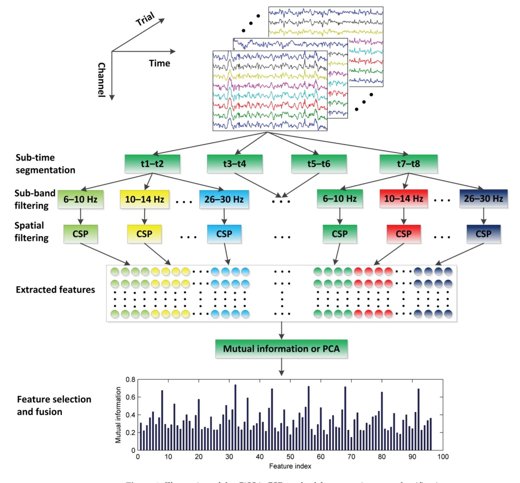
**Figure 1.** Illustration of the CiSSA-CSP method for motor-imagery classification.
68
*Sensors* **2022**, *22*, 8526
#### 2.1. Time Segmentation of EEG Signal
MI EEG signals have distinct temporal behavior and a transient nature [22]. CSP features extracted from the whole time period do not carry any temporal information as EEG signals are averaged over time to compute the covariance matrix. Therefore it is crucial to select the optimal time window and focus on the local properties of the EEG. In order to combine the temporal information in the CSP features, the raw EEG signals are segmented into *T* segments with overlapping time using a sliding window of length 2 s, which can discriminate different motor imagery stages.
#### 2.2. Sub-Band Filtering Using CiSSA
In order to further combine the spectral information in the CSP features, the subbands are composed using the CiSSA method to perform bandpass filtering on all time segments. The CiSSA method is a nonparametric signal extraction method proposed by Juan Bógalo [\[30\]](#30). The CiSSA is derived from the singular spectrum analysis (SSA), which can suppress noise and artifacts with overlapping frequencies compared with the narrowband filter methods such as FIR and IIR [\[17\]](#17). It can decompose the signal into a set of reconstructed components (RCs) of known frequencies. CiSSA consists of four steps: embedding, decomposition, diagonal averaging, and grouping. In the time-delay embedding step, every single-channel EEG time series **s** = ( $s_1, s_2, ..., s_N$ ) $T$ (superscript $T$ denotes the transpose of a vector) is mapped onto a multidimensional trajectory matrix **X** using a sliding window with the window length *L*. In the decomposition step, the trajectory matrix is decomposed into elementary matrices of rank 1 that are associated with different frequencies. To do so, a related circulant matrix **C** $L$ is built based on the second order moments of the time series [\[30\]](#30):
$$\mathbf{C}_{L}(f) = \begin{pmatrix} c_{0} & c_{1} & c_{2} & \cdots & c_{L-1} \\ c_{L-1} & c_{0} & c_{1} & \cdots & c_{L-2} \\ \vdots & \vdots & \vdots & \vdots & \vdots \\ c_{1} & c_{2} & c_{3} & \cdots & c_{0} \end{pmatrix}$$
(1)
where:
$$c_m = \frac{L - m}{L} \gamma_m + \frac{m}{L} \gamma_{L-m}, \quad \gamma_m = \frac{1}{N - m} \sum_{t=1}^{T - m} s_t s_{t+m}, \quad m = 0, 1, \dots, L - 1$$
(2)
The eigenvalues and eigenvectors of **C***L*, respectively, are given by [31]:
$$\lambda_{k} = \sum_{m=0}^{L-1} c_{m} \exp(i2\pi m \frac{k-1}{L}) = f(\frac{k-1}{L})$$
$$\mathbf{u}_{k} = L^{-1/2}(u_{k,1}, u_{k,2}, \dots, u_{k,L})^{H}, \ k = 1, 2, \dots, L$$
$$u_{k,j} = \exp(-i2\pi (j-1)\frac{k-1}{L}), \ j = 1, 2, \dots, L$$
(3)
where *f*(•) denotes the power spectral density of the signal. *H* indicates the conjugate transpose of a matrix. The *k*-th eigenvalue and corresponding eigenvector is associated with the specific frequencies given by:
$$f_k = \frac{k-1}{L} f_s \tag{4}$$
where *fs* is the sampling rate of EEG signals.
Then, in the diagonal averaging step [32], several time series are reconstructed from the elementary matrices. The reconstructed time series are generally called RCs. Thus the raw EEG signal is decomposed into several RCs of known frequency given by Equation (4). The frequency bandwidth of each RC can be roughly expressed by [33]:
69
*Sensors* **2022**, *22*, 8526
$$f_b = f_s / L \tag{5}$$
As a consequence, the frequency bandwidth of each RC is limited to *fs*/*L*. Considering the frequency of each RC given by Equation (4), there is no frequency mixing between different RCs.
We perform bandpass filtering on all time segments using the CiSSA method to obtain a set of non-overlapping sub-bands (*f b*1, *f b*2, ... , *f bB*). These sub-bands are chosen from the frequency range 6–30 Hz with bandwidth of *fb* = 4 Hz, i.e., *f b*1 = 6–10 Hz, *f b*2 = 10–14 Hz, ..., *f bB* = 26–30 Hz where *B* = 6. Then, feature extraction is performed on every sub-band using CSP.
#### 2.3. Feature Extraction Using Common Spatial Patterns
Consider two classes of EEG signal **X***i*,1 and **X***i*,2 *RC*×*P* recorded from the *i*-th trial, where *C* is the number of channels, and *P* denotes the number of sample points. The spatial covariance matrix ∑ of the class *l* (*l* = 1, 2) is given by:
$$\Sigma_{l} = \frac{1}{N_{l}} \sum_{i=1}^{N_{l}} \frac{\mathbf{X}_{i,l} \mathbf{X}_{i,l}^{T}}{trace(\mathbf{X}_{i,l} \mathbf{X}_{i,l}^{T})}$$
(6)
where *Nl* is the number of trials in class *l*. CSP aims at finding linear transforms (spatial filters) to maximize discrimination between two classes [16]. In order to achieve maximum separability between the variance of two classes, the Rayleigh quotient *J*(**w**) is introduced:
$$\max_{\mathbf{w}} J(\mathbf{w}) = \frac{\mathbf{w}^T \mathbf{\Sigma}_1 \mathbf{w}}{\mathbf{w}^T \mathbf{\Sigma}_2 \mathbf{w}} s.t. \left| \left| \mathbf{w} \right| \right|_2 = 1$$
(7)
where ||•||2 denotes the *l*2-norm and **w** ∈ *RC* is a spatial filter. The maximization of Rayleigh quotient *J*(**w**) can be achieved by solving the generalized eigenvalue problem: **Σ**1**w** = *λ***Σ**2**w**. The learned linear transforms (spatial filters) matrix **W** = [**w**1, **w**2, ··· , **w**2*M*] can be obtained by collecting eigenvectors corresponding to the *M* largest and smallest generalized eigenvalues, which represent maximum discrimination between two classes. The spatial filtered EEG, which is the projection **Z** of EEG signal **X**, is then given by **Z** = **W***T***X**.
The variance based CSP feature vector is then formed as **F** = [**F**1, **F**2, ··· , **F**2*M*], where *M* = 2, **F***i* is given by [11]:
$$\mathbf{F}_i = \log(\operatorname{var}(\mathbf{Z}_i)) \tag{8}$$
where var(**Z***i*) denotes the variance of *i*-th row of **Z**.
CSP is implemented on the segmented and filtered signals in each sub-band to calculate the corresponding features by Equation (8). As a result, 2*MBT* = 96 features are extracted from each EEG sample.
#### 2.4. Feature Fusion
The method described above leads to a high-dimension feature set (dimension = 96) that is highly correlated. Obviously using all features for the final decision is not very efficient due to over-learning problems in high dimensions [13]. Therefore, dimension fusion steps are needed to reduce the feature dimensions and improve the performance of classification. We studied two common approaches to obtain a lower dimensionality subset and use them for final classification, namely, mutual information for feature selection and PCA for dimensionality reduction. We feed the reduced feature space to the support vector machine (SVM) and investigate the performance of EEG classification.
70
*Sensors* **2022**, *22*, 8526
#### 2.4.1. Mutual Information
The mutual information-based individual feature (MIBIF) algorithm is a feature selection method that shows good performance in the CSP-based method [34]. For the feature vector set **F** = {**F**1, **F**2,..., **F***d*}, *d* = 2*MBT*, and the corresponding class label Ω = {1, 2}, the mutual information of each feature is calculated:
$$I(\mathbf{F}_i;\Omega) = H(\Omega) - H(\Omega|\mathbf{F}_i), i = 1, 2, \dots, d$$
(9)
where $H(\Omega) = -\sum_{\omega=1}^{2} p(\omega) \log_{2} p(\omega), \omega \in \Omega$ , the conditional entropy is:
$$H(\Omega|\mathbf{F}_i) = -\sum_{\omega=1}^{2} p(\omega|\mathbf{F}_i) \log_2 p(\omega|\mathbf{F}_i)$$
(10)
A higher magnitude of mutual information means more relevance between the feature and the class. Thus, the features are ranked in descending order according to mutual information and the top *k* significant features are selected.
#### 2.4.2. PCA
PCA is a useful approach to decorrelate the features and reduce the dimensionality of the feature space [35]. The purpose of PCA is to find the linear orthogonal transformation matrix that maximally maintains the feature variance [36]. The mean feature vector **m***v* = ∑*n i*=1 **f***i*/*n* is calculated from the feature vector set **F** = [**f**1,**f**2, ··· ,**f***d*], *d* denotes the number of features. Then, covariance matrix **C**PCA for **F** is calculated as follows:
$$\mathbf{C}_{\text{PCA}} = \frac{1}{n-1} \sum_{i=1}^{d} (\mathbf{f}_{i} - \mathbf{m}_{v}) (\mathbf{f}_{i} - \mathbf{m}_{v})^{T}$$
(11)
The PCA projection matrix **W**PCA can be obtained by calculating the eigenvectors and eigenvalues for the covariance matrix and selecting the top *k* columns of eigenvectors in descending order of eigenvalue sizes.
#### 3. Data and Experiment
In order to better verify the validity of the proposed CiSSA-CSP method, we used two different MI EEG datasets for analysis. The first dataset was the BCI Competition III dataset IVa, which is publicly available and has been used in many studies [34,37]. Therefore, using this dataset, we can effectively compare our method with competing methods. In addition, in order to verify the universal applicability of the method, the second dataset, which was collected by ourselves, was used for analysis and validation.
#### 3.1. Public EEG Dataset
BCI Competition III dataset IVa was recorded from five healthy subjects (subject aa, al, av, aw, and ay). The subjects sat in a comfortable chair and performed motor imagery (right hand and right foot) experiments. The EEG signal was recorded using 118 channels according to the extended international 10–20 system and 140 trials for each class. Thus, a total of 280 trials were provided for each subject. The sampling rate of the EEG data was 100 Hz. Each trial lasted 3.5 s of motor imagery and was interrupted by a time period of 1.75 to 2.25 s, in which the subject could relax, shown in Figure 2b. Seventeen EEG channels were selected in our study, as shown in Figure 2a (FC3, FC1, FCz, FC2, FC4, C5, C3, C1, Cz, C2, C4, C6, CP3, CP1, CPz, CP2, CP4), which contain the sensorimotor area needed to recognize the cue in the experiment [34].
#### 3.2. Experimental EEG Dataset
The experiments were approved with a protocol (NO. 20170010) by the Institutional Review Board of Tsinghua University and written informed consent was obtained from the subjects. Twenty healthy subjects (subject S1, S2, ... , S20) aged 20–29 participated in 71
*Sensors* **2022**, *22*, 8526
the experiments and abstained from psychoactive substances for at least 4 h prior to the experiments. The experiments were carried out with the subjects sitting on a comfortable chair in a room with normal lightness. The experimental EEG signals were recorded with nine electrodes (F3, Fz, F4, C3, Cz, C4, P3, Pz, P4) from the international 10–20 system, shown in Figure 3a, using the MP160 data acquisition and analysis system (BIOPAC Systems, Inc., Goleta, CA, USA). During each trial, as shown in Figure 3b, the subject relaxed for 3 s, and then a visual cue was presented. Two seconds later, the subject performed the right-hand or right-foot motor imaginary tasks for 5 s. There were 140 trials for each class per subject, i.e., a total of 280 trials for each subject. All EEG signals were recorded at a sampling rate of 250 Hz.
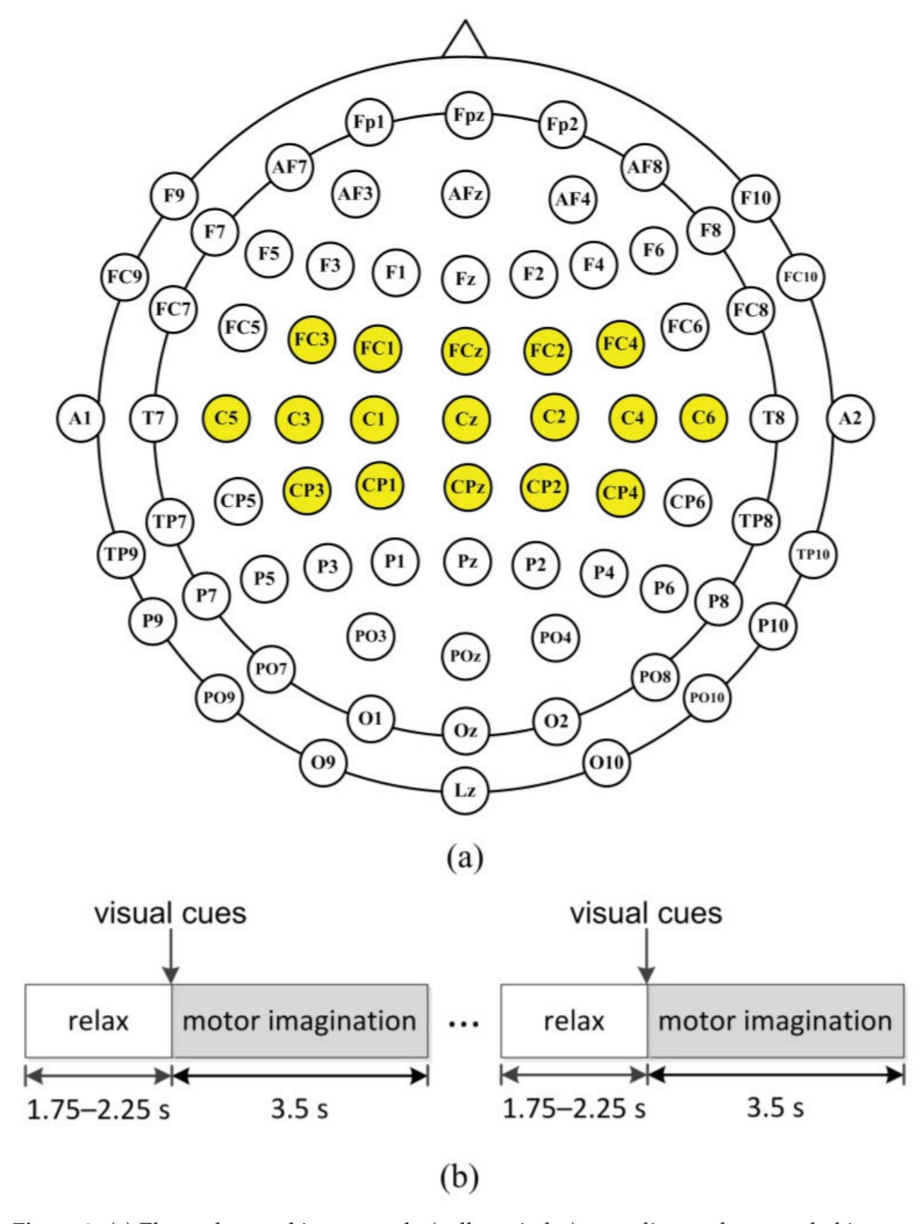
**Figure 2.** (**a**) Electrodes used in our study (yellow circles) according to the extended international 10–20 system. (**b**) The scheme of the experiment. A single trial of the experiment was divided into two periods. In the first period, the subject relaxed for 1.75–2.25 s; and then the visual cues were indicated for 3.5 s when the subject performed the motor imageries.
72
*Sensors* **2022**, *22*, 8526
**Figure 3.** Experiment setup. (**a**) Electrodes used in the experiment (yellow circles) according to the international 10−20 system. (**b**) The scheme of the experiment. A single trial of the experiment was divided into three periods. In the first period, the subject relaxed for 3 s; and then the visual cues were indicated for 2 s for preparation. Finally, subjects performed the motor-imagery tasks (right hand or foot) for 5 s.
#### 4. Results and Discussion
#### 4.1. Results and Discussion of Public EEG Dataset
The 17-channel EEG signals of all trials were segmented into *T* = 4 segments with overlapping time of 1.5 s (0–2 s, 0.5–2.5 s, 1–3 s, 1.5–3.5 s). Then, every time segment was bandpass filtered into *B* = 6 sub-bands without overlapping frequency using the CiSSA method (6–10 Hz, 10–14 Hz, 14–18 Hz, 18–22 Hz, 22–26 Hz, 26–30 Hz). A total of 2*M* = 4 features were extracted from every sub-band by CSP and, thus, 2*MBT* = 96 features were obtained. Finally, dimension reduction was conducted by mutual information or PCA and optimal features are selected for MI classification. A 10-fold cross-validation was implemented to evaluate the classification performance.
Table 1 shows the classification accuracy of different algorithms for five subjects using 10-fold cross-validation. The classification performance of standard CSP is not very good, especially for subject aa, av, and aw. The average classification accuracy of CSP is 81.6%. We refer to classification results obtained with CiSSA filtered sub-bands before CSP as CiSSA + CSP. Classification results indicated that CiSSA + CSP provides improvements compared to CSP for all subjects, especially for aa, av, and aw. The average classification accuracy of CiSSA + CSP is 92.3%, which is much higher than the accuracy of CSP. This proves that combining spectral information in the CSP features can greatly improve the performance of MI classification. The results corresponding to the Subtime + CiSSA + CSP are obtained with time segmentation processing before CiSSA + CSP. With the exception of subject aw, the classification accuracy increases with all subjects when time
73
*Sensors* **2022**, *22*, 8526
segmentation is implemented. The average accuracy of Subtime + CiSSA + CSP increases to 94.5%, proving that combining temporal information in the CSP features can further improve the classification accuracy of MI EEG. The results obtained with MIBIF and PCA processing as dimensionality reduction are referred as Subtime + CiSSA + CSP + MIBIF and Subtime + CiSSA + CSP + PCA, respectively. Note that *k* = 9 optimal features are selected for all subjects to preliminary study the effects of MIBIF and PCA. When MIBIF is used as the feature selection method, the classification accuracy decreases for subjects aa, al, and av, and the average classification accuracy decreases to 93.6%. This indicates that nine optimal features are not enough to carry sufficient discriminative information. Further studies should be conducted to select suitable and optimal features. When PCA is used for dimensionality reduction, the classification accuracy increases slightly with all subjects except for subject aa. Subtime + CiSSA + CSP + PCA provides the best results with an average classification accuracy of 96.4%.
**Table 1.** The classification accuracies of the proposed CiSSA-CSP method on BCI Competition III dataset IVa (subject aa, al, av, aw, and ay).
| | Classification Accuracy (%) | | | | | |
|-------------------------------|-----------------------------|------------|-------------|------------|------------|------------|
| Method | aa | al | av | aw | ay | Average |
| CSP | 78.6 ± 11.4 | 96.4 ± 3.8 | 69.6 ± 10.7 | 75.0 ± 6.3 | 88.6 ± 5.0 | 81.6 ± 7.4 |
| CiSSA + CSP | 94.3 ± 5.9 | 98.2 ± 3.5 | 78.6 ± 6.5 | 98.2 ± 2.5 | 92.4 ± 4.1 | 92.3 ± 4.5 |
| Subtime + CiSSA + CSP | 98.6 ± 1.8 | 99.3 ± 1.5 | 83.2 ± 6.1 | 97.9 ± 3.0 | 95.7 ± 2.8 | 94.9 ± 3.0 |
| Subtime + CiSSA + CSP + MIBIF | 94.3 ± 6.6 | 98.2 ± 1.9 | 79.6 ± 7.4 | 98.2 ± 2.5 | 97.9 ± 3.8 | 93.6 ± 4.4 |
| Subtime + CiSSA + CSP + PCA | 98.2 ± 3.0 | 99.3 ± 1.5 | 87.5 ± 7.6 | 100 ± 0 | 97.1 ± 2.8 | 96.4 ± 3.0 |
#### 4.1.1. Discriminative Frequency Sub-Band Features
In order to understand the effect of the combination of spectral information with CSP features, we visualized the topographical distribution of the broad band and the subband EEGs. Figure 4 presents the topographical map and the filter coefficient of the most significant spatial filter learned by the CSP method from the broad band and all sub-bands for subject av. Only the electrodes of the sensorimotor area (inside the red dotted frame) are presented in the topographical map. A larger absolute value of the filter coefficient means more discriminative information [16]. It can be seen that the largest filter coefficient of the most significant spatial filter in the broad frequency band (6–30 Hz) is only 0.44, which leads to poor separability. The largest filter coefficients of the most significant spatial filter in sub-bands 6–10 Hz, 10–14 Hz, 14–18 Hz, 18–22 Hz, 22–26 Hz, and 26–30 Hz are −0.46, 0.43, 0.6, 0.66, 0.59 and 0.77, respectively. This indicates better separability in Beta rhythm sub-bands (14–18 Hz, 18–22 Hz, 22–26 Hz, and 26–30 Hz) than in Mu rhythm sub-bands (6–10 Hz and 10–14 Hz) and broad band (6–30 Hz) for subject av. More discriminative spectral information is combined in the Beta rhythm sub-bands features. Therefore, we need to find more precise frequency sub-bands for MI CSP feature extraction, since these sub-bands carry the most discriminative information and the remaining sub-bands are irrelevant and redundant to the MI tasks. It is concluded that the combination of spectral information in the CSP features by an effective optimization of filter band is necessary to improve the MI classification performance.
In the study, the sub-bands of the EEG were extracted by the CiSSA. In order to compare the performance of sub-band extraction and classification with other common filtering methods, the sub-bands were extracted by FIR filtering with order 60, Butterworth IIR filtering with order 7, and the wavelet decomposition (WDec) methods, and the classification accuracies were calculated on CSP features extracted from these sub-bands. Furthermore, the independent component analysis (ICA) method is commonly used in signal decomposition and artifact removal of EEG [38]. The noise and artifacts are removed by the FastICA method based on Negentropy [38] and then the sub-bands are extracted by FIR filtering. Table 2 shows the classification accuracies of CSP, FIR + CSP, IIR + CSP, WDec + CSP, 74
*Sensors* **2022**, *22*, 8526
ICA + CSP, ICA + FIR + CSP, and CiSSA + CSP methods on BCI Competition III dataset IVa. It can be seen that, compared with the standard CSP on the broad EEG band, the classification accuracies are highly improved for sub-bands by FIR, IIR, WDec and CiSSA. This proves that combining spectral information can greatly improve the discrimination of CSP features. Expert for subject ay, the classification accuracies obtained by CiSSA are higher than those obtained by FIR, IIR, and WDec for all subjects. The average classification accuracy obtained by CiSSA is improved by 2.3%, 2.9%, and 1.9% over the average classification accuracies obtained by FIR, IIR, and WDec, respectively. This is because the CiSSA can suppress noise and artifacts with overlapping frequencies of sub-bands, while the FIR, IIR, and the WDec methods are not able to separate the noise overlapping in the frequency space, which decreases the classification performance of CSP. Figure 5 shows the power spectrum density (PSD) of the sub-bands extracted by CiSSA, FIR, IIR, WDec, and ICA + FIR for subject av at electrode C3. It can be seen that the PSDs of sub-bands extracted by FIR and IIR are higher than those by CiSSA and ICA + FIR, which can suppress noise and artifacts with overlapping frequencies. The PSDs of sub-bands extracted by WDec contain components falling outside the frequency width of sub-bands. Although ICA can also remove noise and artifacts with overlapping frequencies, the average classification accuracy obtained by ICA + FIR is lower than that obtained by CiSSA. It is concluded that the CiSSA extracts more precise frequency sub-bands for MI CSP feature extraction.
**Figure 4.** The topographical map and the filter coefficient of the most significant spatial filter learned by the CSP method of each sub-band for subject av. The electrode indexes 1, 2, ... , 17 correspond to the electrode FC3, FC1, FCz, FC2, FC4, C5, C3, C1, Cz, C2, C4, C6, CP3, CP1, CPz, CP2, CP4, respectively. Electrodes inside the red outline represent the electrode indexes 1, 2, . . . , 17.
75
*Sensors* **2022**, *22*, 8526
**Table 2.** The classification accuracies of FIR + CSP, IIR + CSP, WDec + CSP, ICA + CSP, ICA + FIR + CSP, and CiSSA + CSP methods on BCI Competition III dataset IVa (subject aa, al, av, aw, and ay).
| Classification Accuracy (%) | | | | | | |
|-----------------------------|------------|------------|-------------|------------|------------|------------|
| Method | aa | al | av | aw | ay | Average |
| FIR + CSP | 85.7 ± 8.8 | 95.4 ± 3.8 | 78.6 ± 8.8 | 97.1 ± 2.3 | 93.2 ± 4.6 | 90.0 ± 5.7 |
| IIR + CSP | 87.1 ± 9.9 | 93.9 ± 4.1 | 76.8 ± 12.3 | 97.9 ± 3.0 | 91.4 ± 4.5 | 89.4 ± 6.8 |
| WDec + CSP | 93.9 ± 8.4 | 96.8 ± 3.6 | 72.6 ± 10.4 | 97.9 ± 3.8 | 90.7 ± 4.2 | 90.4 ± 6.1 |
| ICA + CSP | 81.1 ± 6.5 | 95.0 ± 5.1 | 71.1 ± 10.0 | 77.5 ± 6.1 | 94.3 ± 3.5 | 83.6 ± 6.2 |
| ICA + FIR + CSP | 90.4 ± 8.1 | 93.6 ± 2.8 | 81.1 ± 7.7 | 94.3 ± 3.8 | 95.7 ± 2.3 | 91.0 ± 4.9 |
| CiSSA + CSP | 94.3 ± 5.9 | 98.2 ± 3.5 | 78.6 ± 6.5 | 98.2 ± 2.5 | 92.4 ± 4.1 | 92.3 ± 4.5 |
**Figure 5.** The power spectrum density (PSD) of the sub-bands extracted by CiSSA, FIR, IIR, WDec, and ICA + FIR for subject av at electrode C3. The PSDs of sun-bands extracted by FIR and IIR are higher than those by CiSSA and ICA + FIR. The PSDs of sun-bands extracted by WDec contain components falling outside the frequency width (e.g., 6–10 Hz for sub-band1).
The bandwidth of sub-bands is 4 Hz, which is used in most of the previous studies [8,10,12,24,39]. Table 3 shows the classification accuracies of CiSSA + CSP method on different bandwidths on BCI Competition III dataset IVa using 10-fold cross-validation. It can be seen that the classification accuracy attains a high value when the bandwidth is set to be 1 or 4 Hz. However, more computing resources and time are needed for a bandwidth of 1 Hz than for a bandwidth of 4 Hz. Therefore, the bandwidth of 4 Hz is the best choice for sub-band extraction.
#### 4.1.2. The Performance of Time Segmentation
To present time window segmentation performance, we made topoplots of spatial filters for subject aa as an example, shown in Figure 6. Figure 6a shows the classification accuracy of the feature space learned by the proposed CiSSA-CSP method using a pictorial representation. Overall, the feature space has five time windows (the whole time window and four sub-time windows) and six frequency sub-bands for each time window. Each time-frequency segment contains four CSP features. It can be observed that CSP feature index 8 (sub-band 10–14 Hz), index 12 (sub-band 14–18 Hz), and index 20 (sub-band 76
*Sensors* **2022**, *22*, 8526
22–26 Hz), which represent the most significant spatial filters learned by the CSP from the sub-bands, attain the best classification accuracy. Features from CSP feature index 12 in all time windows are marked by a red outline. The classification accuracy of sub-time window 0.5–2.5 s is higher than the accuracies of the whole time window of 0–3.5 s and other sub-time windows of 0–2 s, 1–3 s, and 1.5–3.5 s. To further analyze the effect of the proposed method in different time windows, the topographical maps of the most significant spatial filter learned by the CSP from all time windows in sub-band 14–18 Hz (marked by red outline in Figure 6a) are shown in Figure 6b. An evident change in ERD/ERS patterns in the sensorimotor area is observed as the time window changes, which shows that the neural response during motor imagery tasks changes with time. In sub-time windows 0.5–2.5 s, spatial features are more discriminative and significant than in other sub-time windows and the whole time window. Therefore, combining temporal information into CSP features by time segmentation leads to more discriminatory features for MI task classification.
**Table 3.** The classification accuracies of CiSSA + CSP methods on different bandwidths on BCI Competition III dataset IVa (subject aa, al, av, aw, and ay).
| Bandwidth (Hz) | L | Classification Accuracy (%) | | | | | |
|----------------|-----|-----------------------------|------------|-------------|------------|------------|------------|
| | | aa | al | av | aw | ay | Average |
| 1 | 100 | 93.5 ± 4.1 | 98.2 ± 2.5 | 84.3 ± 7.3 | 91.0 ± 4.8 | 94.1 ± 4.7 | 92.2 ± 4.7 |
| 2 | 50 | 88.3 ± 6.6 | 97.4 ± 2.3 | 79.6 ± 6.7 | 96.4 ± 2.8 | 92.3 ± 6.3 | 90.8 ± 4.9 |
| 4 | 25 | 94.3 ± 5.9 | 98.2 ± 3.5 | 78.6 ± 6.5 | 98.2 ± 2.5 | 92.4 ± 4.1 | 92.3 ± 4.5 |
| 6 | 16 | 90.7 ± 6.1 | 97.5 ± 2.9 | 78.9 ± 11.0 | 97.1 ± 2.8 | 94.3 ± 4.8 | 91.7 ± 5.5 |
| 8 | 12 | 88.6 ± 9.3 | 98.6 ± 1.8 | 73.6 ± 9.7 | 92.9 ± 4.8 | 92.5 ± 3.9 | 89.2 ± 5.9 |
**Figure 6.** Performance of time segmentation for subject aa. (**a**) Pictorial representation of the classification accuracy (ACC) on the feature space learned by the proposed method for subject aa. Each time-frequency segment contains 4 CSP features. (**b**) The topographical maps of the most significant spatial filter learned by the CSP from all time windows in sub-band 14–18 Hz (marked by red outline in Figure 6a). Electrodes inside red outline in Figure 6b represent the electrodes of the sensorimotor area.
77
*Sensors* **2022**, *22*, 8526
The performance of classification is affected by time-window length. The classification accuracies at different time-window lengths with a window step of 0.5 s were calculated using 10-fold cross-validation and the results are shown in Table 4. It can be seen that the classification accuracies vary within a small range of 1.2% and the accuracy attains a maximum value at time-window length of 2 s.
**Table 4.** The classification accuracies at different time-window lengths on BCI Competition III dataset IVa (subject aa, al, av, aw, and ay).
| Time-Window Length (s) | Classification Accuracy (%) | | | | | |
|------------------------|-----------------------------|------------|------------|------------|------------|------------|
| | aa | al | av | aw | ay | Average |
| 1 | 98.3 ± 2.4 | 100 | 79.9 ± 3.8 | 96.1 ± 1.7 | 94.3 ± 2.4 | 93.7 ± 2.1 |
| 1.5 | 96.5 ± 2.5 | 99.6 ± 1.1 | 85.3 ± 5.4 | 97.6 ± 1.1 | 94.3 ± 1.5 | 94.7 ± 2.3 |
| 2 | 98.6 ± 1.8 | 99.3 ± 1.5 | 83.2 ± 6.1 | 97.9 ± 3.0 | 95.7 ± 2.8 | 94.9 ± 3.0 |
| 2.5 | 96.8 ± 2.6 | 99.0 ± 1.1 | 82.5 ± 8.0 | 97.9 ± 3.0 | 91.1 ± 5.1 | 93.5 ± 4.0 |
| 3 | 97.1 ± 2.8 | 99.0 ± 1.5 | 81.1 ± 6.1 | 97.5 ± 3.4 | 92.9 ± 6.1 | 93.5 ± 4.0 |
#### 4.1.3. The Effect of Feature Selection by MIBIF
To have an intuitive understanding of the distribution of significant time-frequency segments, the values of MIBIF belonging to each time-frequency segment were calculated, as shown in Figure 7 for subject aa. It can be seen that the highest values are located in feature indexes 8, 12, and 20, which is consistent with Figure 6. It is concluded that the features of higher MIBIF values contain more discriminatory information for accuracy improvement of MI EEG. In addition, the significance (MIBIF value) changes along the time axis and frequency bands due to the non-stationarity of EEG. The most significant features are located in some local time-frequency segments. Therefore, it is believed that decomposing a multi-channel EEG into time-frequency segments for more precise analysis helps to improve the classification accuracy. Figure 8 depicts distributions of the most significant two features derived by CSP, CiSSA + CSP, Subtime + CSP, and Subtime + CiSSA + CSP, for subject aa. It is indicated that when the spectral (CiSSA + CSP) or temporal (Subtime + CSP) information is combined into the CSP features, more separable feature distributions are provided in comparison with the standard CSP. The highest discriminability of features was achieved by Subtime + CiSSA + CSP, which combines both the spectral and temporal information. The classification accuracy of the two most significant features derived by Subtime + CiSSA + CSP is 85.0%, 10.7% higher than the classification accuracy obtained by standard CSP.
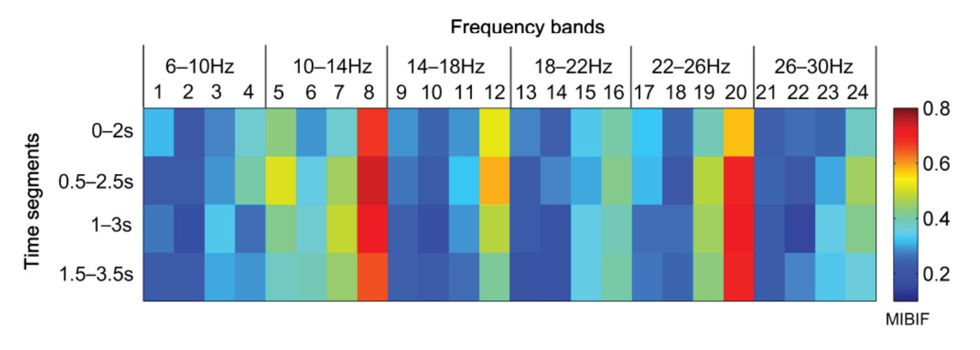
**Figure 7.** Distribution of MIBIF values in all time-frequency segments for subjects aa. Index 1, 2, ... , 24 in the frequency bands represent the CSP feature index.
The classification accuracy of the proposed mothed varies with the number of the features selected by the MIBIF. To select the most suitable features, the classification accuracies for the number of selected features by MIBIF were calculated, as shown in Figure 9 for subject av. Figure 9 indicates that the highest classification accuracy (85.7%) is attained
78
*Sensors* **2022**, *22*, 8526
when the most significant 25 features are selected for subject av. The highest classification accuracies and the number of selected features by MIBIF for all subjects are shown in Table 5. The average highest classification accuracy with feature selection by MIBIF for all subjects is 96.3%, which is a 1.4% improvement compared to the average classification accuracy without feature selection.
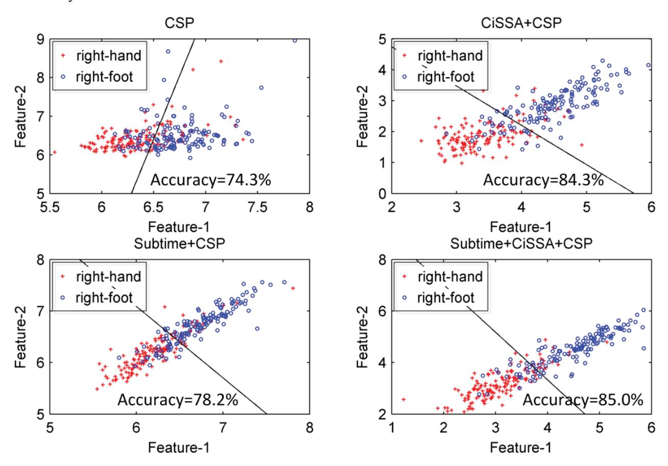
**Figure 8.** Distributions of the most two significant features obtained by CSP, CiSSA + CSP, Subtime + CSP and Subtime + CiSSA + CSP, for subjects aa.
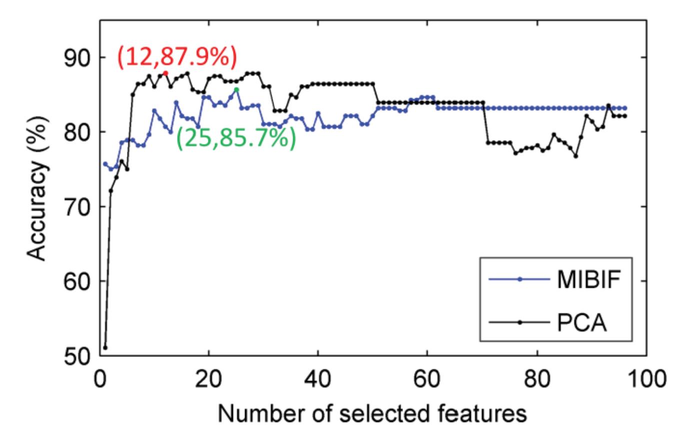
**Figure 9.** Classification accuracy over the number of selected features by MIBIF and PCA for subjects av.
#### 4.1.4. The Effect of Dimensionality Reduction by PCA
We note from Table 1 that the classification accuracies are increased when features are dimensionally reduced by PCA for certain subjects (av, aw, and ay). The receiver operating characteristic (ROC) curves related to the 57 features selected by MIBIF and five features selected by PCA for subject aa are given in Figure 10a. It is indicated that the area under 79
*Sensors* **2022**, *22*, 8526
the PCA curve is greater than the areas under curves of selected MIBIF features and all the original features, which means more discrimination in the selected features by PCA than by MIBIF. Figure 10b shows the distribution of the first two features obtained by PCA for subject aa. Note that the right-hand and -foot imagery classes are nearly linearly separable with the top two features with PCA. The classification accuracy of the first two features derived by PCA is 93.6%, higher than the classification accuracy derived by MIBIF (shown in Figure 8).
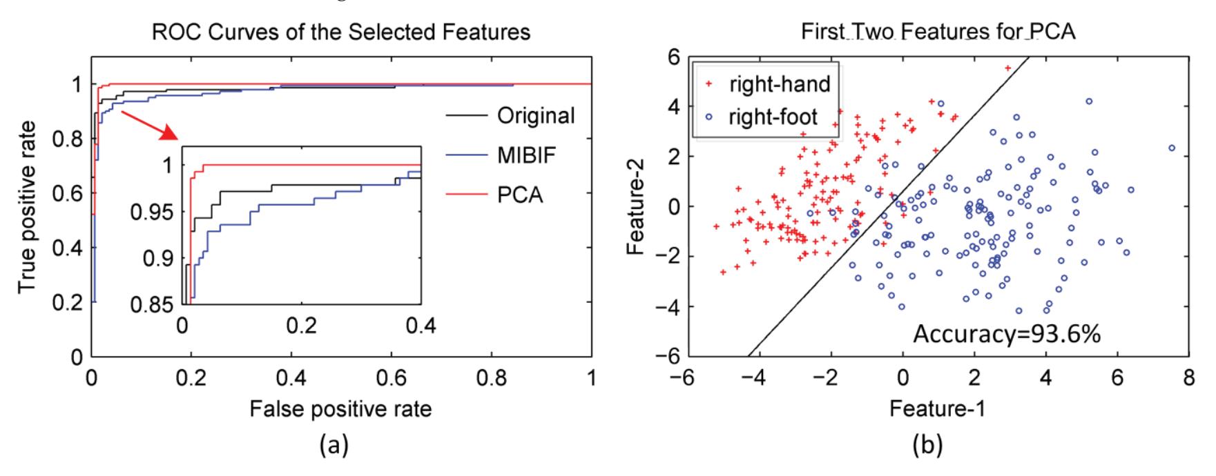
**Figure 10.** (**a**) The ROC curve of the 57 features selected by MIBIF and 5 features selected by PCA for subjects aa. (**b**) The distribution of the first two features obtained by PCA for subject aa. Note that the right-hand (blue, circle) and right-foot (red, cross) imagery classes are nearly linearly separable with only 2 features.
Similar to MIBIF, the classification accuracy also varies with the feature dimension selected by the PCA. It is indicated by Figure 9 that the highest classification accuracy (87.9%) is attained when the most significant 12 features derived by PCA are selected for subject av. The classification accuracy of PCA is higher than that of MIBIF when the same number of top significant features is selected. This is because PCA can decorrelate the features and reduce the redundant information between features, while MIBIF extracts features most relevant to the class. Features extracted by MIBIF may be highly correlated and contain redundant information. Figure 11 shows the distribution of mutual information between top 25 features selected by MIBIF and PCA for subject av. A higher value of mutual information means more relevance between two features. It can be seen that the top features extracted by MIBIF are highly correlated, while the features extracted by PCA are not correlated. The highest classification accuracies and the selected feature dimension by PCA for all subjects are shown in Table 5. The average highest classification accuracy with dimensionality reduction by PCA for all subjects is 96.6%, 0.3% higher than the accuracy derived by MIBIF.
**Table 5.** The highest classification accuracies and the selected feature dimension (*k*) by MIBIF and PCA for all subjects on Competition III dataset IVa (subject aa, al, av, aw, and ay).
| Subject | MIBIF | | PCA | |
|---------|--------------|---------------|--------------|---------------|
| | Accuracy (%) | Dimension (k) | Accuracy (%) | Dimension (k) |
| aa | 98.6 ± 1.8 | 57 | 98.2 ± 2.5 | 5 |
| al | 99.6 ± 1.1 | 28 | 99.6 ± 1.1 | 11 |
| av | 85.7 ± 7.9 | 25 | 87.9 ± 6.8 | 12 |
| aw | 99.6 ± 1.1 | 10 | 100 | 9 |
| ay | 97.9 ± 3.8 | 8 | 97.5 ± 4.7 | 16 |
| Average | 96.3 ± 3.1 | | 96.6 ± 3.0 | |
80
*Sensors* **2022**, *22*, 8526
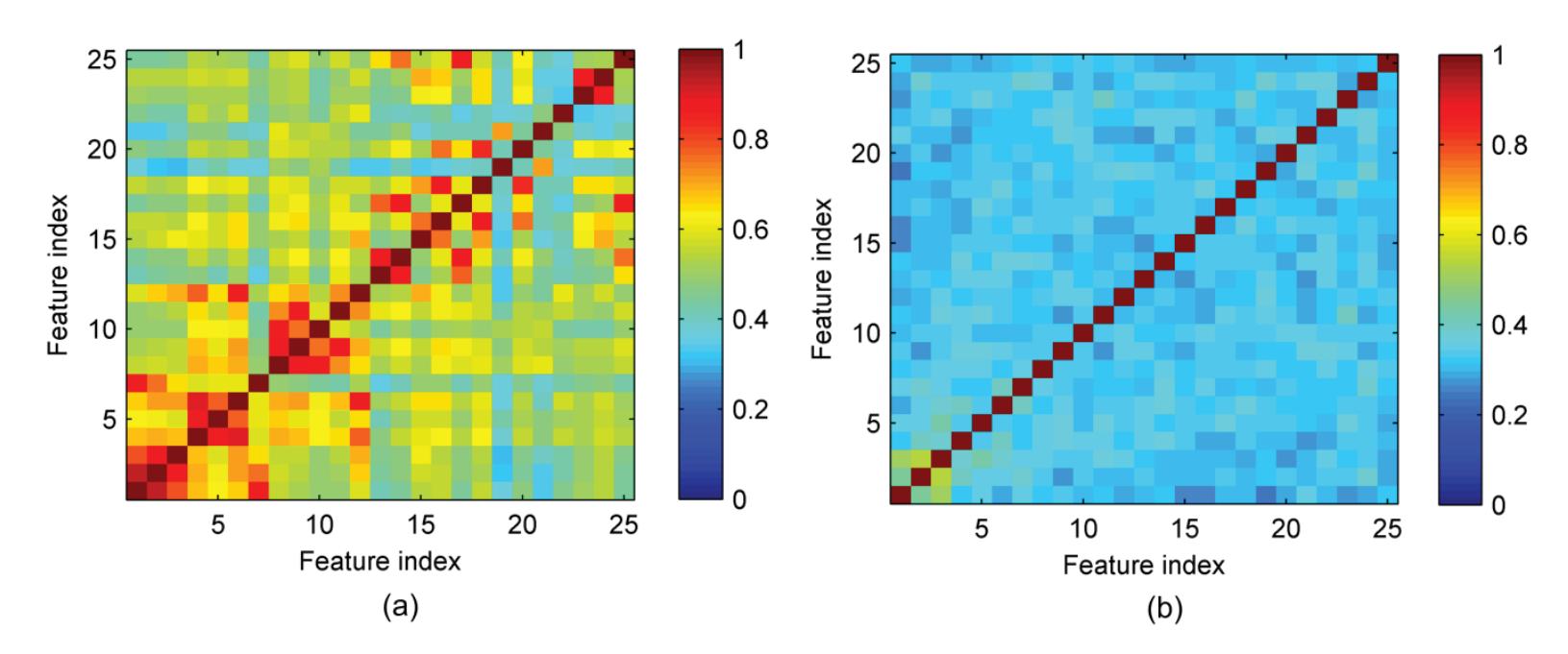
**Figure 11.** The distribution of mutual information between the top 25 features selected by (**a**) MIBIF and (**b**) PCA for subject av.
#### 4.1.5. Comparison with Other Competing Techniques
Since accuracy is the key criterion for evaluating the performance of methods in a BCI system, we compared the classification accuracy of the proposed CiSSA-CSP method with other competing methods. Table 6 provides a comparative study of the classification performance between the proposed method and ten recently reported methods for Competition III dataset IVa, namely, FBCSP [14], CTFSP [6], Fusion [18], TWFBCSP-MVO [24], SFBCSP [16], STFSCSP [39], DFBCSP [40], CC-LR [37], ISSPL [41], and Class Separability (CS) [35] methods. The highest classification accuracies among these methods are highlighted in bold font for each subject and their averages. The highest classification accuracy of our proposed method is 100% for subject aw. Furthermore, the classification accuracies of our proposed method for subjects aa, al, and ay are very close to the highest classification accuracy of other competing methods. The average classification accuracies of our proposed method are 96.3% and 96.6% for MIBIF and PCA feature selection, respectively, which are higher than the average classification accuracies of other methods. It can be concluded that the proposed method outperforms the recently reported competing methods for MI EEG classification.
**Table 6.** Comparison of the classification performance between the proposed method and eight recently reported methods for Competition III dataset IVa (subject aa, al, av, aw, and ay).
| Method | Classification Accuracy (%) | | | | | |
|-------------------------|-----------------------------|------|------|------|------|---------|
| | aa | al | av | aw | ay | Average |
| FBCSP [14] | 83.6 | 94.6 | 51.4 | 93.9 | 88.2 | 82.4 |
| CTFSP [6] | 86.1 | 98.6 | 52.1 | 96.1 | 92.1 | 85.0 |
| Fusion [18] | 80.0 | 96.8 | 70.0 | 92.5 | 91.1 | 86.1 |
| TWFBCSP-MVO [24] | 89.6 | 99.3 | 69.3 | 96.1 | 92.1 | 89.3 |
| SFBCSP [16] | 91.5 | 98.6 | 77.4 | 98.0 | 94.7 | 92.0 |
| STFSCSP [39] | 92.5 | 98.6 | 79.4 | 97.8 | 95.0 | 92.7 |
| DFBCSP [40] | 92.3 | 99.3 | 78.1 | 99.3 | 95.1 | 92.8 |
| CC-LR [37] | 100 | 94.2 | 100 | 100 | 75.3 | 93.9 |
| ISSPL [41] | 93.6 | 100 | 79.3 | 99.6 | 98.6 | 94.2 |
| Class Separability [35] | 95.6 | 99.7 | 90.5 | 98.4 | 95.7 | 96.0 |
| Our method (MIBIF) | 98.6 | 99.6 | 85.7 | 99.6 | 97.9 | 96.3 |
| Our method (PCA) | 98.2 | 99.6 | 87.9 | 100 | 97.5 | 96.6 |
#### 4.1.6. Computational Complexity
In order to investigate the computational complexity of the proposed method, we calculated the time consumption of training and testing phase on Competition III dataset 81
*Sensors* **2022**, *22*, 8526
IVa. The experiment was implemented using MATLAB R2014a on a PC with Intel(R) Core(TM) 2.40 GHz CPU and 8.0 GB RAM. Figure 12 shows the computational time of the training phase taken by different methods with 10-fold cross-validation. From Figure 12a, it can be seen that combining spectral and temporal information in the CSP features by sub-band filtering (CiSSA + CSP) and time segmentation (Subtime + CiSSA + CSP) takes much more time than the CSP method. In addition, the time required by the MIBIF feature selection method is much longer than PCA. Furthermore, we compared the time consumption of CiSSA and other common filtering methods, as shown in Figure 12b. The results indicate that CiSSA and FIR consume the least time, while CiSSA achieves the highest classification accuracy (shown in Table 2).
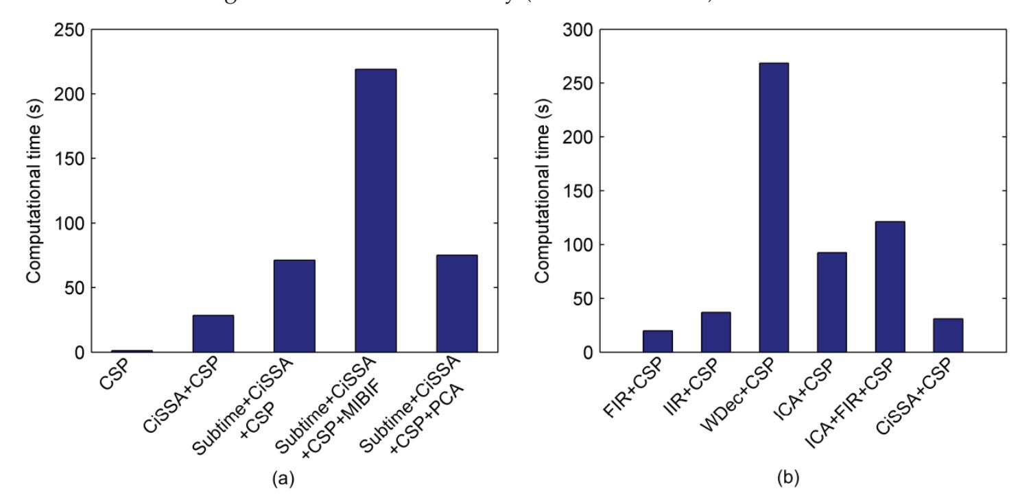
**Figure 12.** Computational time taken by different methods on Competition III dataset IVa with 10-fold cross-validation. (**a**) Computational time taken by CSP, CiSSA + CSP, Subtime + CiSSA + CSP, Subtime + CiSSA + CSP + MIBIF and Subtime + CiSSA + CSP + PCA. (**b**) Computational time taken by FIR + CSP, IIR + CSP, WDec + CSP, ICA + CSP, ICA + FIR + CSP and CiSSA + CSP.
After training, the optimal CSP filter for each time-frequency segment, the indexes of selected features, and the SVM model can be directly used for testing. Hence the computational time is significantly reduced during the testing phase. Table 7 lists the average testing time of one trial using our method and other recently reported methods for subject aa. The results indicate that, for one test trial, the average execution time of our method is 156.4 ms (MIBIF) or 156.7 ms (PCA). Although our method takes a longer time to compute one trial than other competing methods, it can meet the requirement of real-time processing since the computational time is much less than the length of one trial (3.5 s). Therefore, the proposed method improves the motor imagery classification performance without degrading the computation efficiency for BCI applications.
**Table 7.** Comparison of average computational time for testing one trial with different competing methods for subject aa.
| Methods | Testing Time (ms) |
|--------------------|-------------------|
| FBCSP | 78.8 |
| CTFSP | 143.2 |
| DFBCSP | 146.6 |
| Fusion | 23.4 |
| STFSCSP | 45.2 |
| Class Separability | 72.6 |
| Our method (MIBIF) | 156.4 |
| Our method (PCA) | 156.7 |
82
*Sensors* **2022**, *22*, 8526
#### 4.2. Results and Discussion of Experimental EEG Dataset
In the study of the experimental EEG dataset, the 9-channel EEG signals of all trials were segmented into *T* = 4 epochs with overlapping time of 1s (0–2 s, 1–3 s, 2–4 s, 3–5 s). Table 8 shows the classification accuracies of different algorithms for twenty subjects using 10-fold cross-validation. The classification performance of CSP is poor for most subjects and the average accuracy of CSP is 74.7%. When spectral information is combined with the CSP features by decomposing the EEG into sub-bands using CiSSA, the classification performance improves compared to CSP for all subjects. The average classification accuracy of CiSSA + CSP is 90.4%. The average accuracy of Subtime + CiSSA + CSP further increases to 92.3%. Similar to the public available dataset, *k* = 9 optimal features were selected for all subjects to preliminarily study the effects of MIBIF and PCA. When MIBIF is used as the feature selection method after Subtime + CiSSA + CSP, the classification accuracy decreases for most subjects and the average classification accuracy decreases to 89.8%, indicating that nine optimal features are not enough to carry sufficient discriminative information. When PCA is used for dimensionality reduction after Subtime + CiSSA + CSP, the classification accuracy increases slightly with all subjects, except for subjects S1, S12, and S14. Subtime + CiSSA + CSP + PCA provides the best results with an average classification accuracy of 93.9%. The results of the experimental EEG dataset are consistent with the results of Competition III dataset IVa. It is concluded that the proposed CiSSA-CSP method can be used in different MI datasets, which verifies the universal applicability of the method. To verify the reliability of the experimental results, a paired *t*-test [27] is used between two adjacent methods in Tables 1 and 8 to show the statistical difference in the classification accuracies of different methods. The paired *t*-test's results on all subjects of public and experimental datasets are shown in Table 9. It can be seen that all the *p*-values are less than 0.05 (*p* < 0.05), which means all improvements are statistically significant.
**Table 8.** The classification accuracies of the proposed CiSSA-CSP method on experimental motor imaginary EEG.
| | Classification Accuracy (%) | | | | | |
|---------|-----------------------------|-------------|-------------------------|---------------------------------|-------------------------------|--|
| Subject | CSP | CiSSA + CSP | Subtime + CiSSA
+CSP | Subtime + CiSSA
+CSP + MIBIF | Subtime + CiSSA
+CSP + PCA | |
| S1 | 70.4 ± 6.1 | 97.5 ± 2.9 | 96.4 ± 4.1 | 93.6 ± 5.0 | 95.4 ± 4.5 | |
| S2 | 68.2 ± 10.6 | 87.5 ± 5.1 | 91.4 ± 3.0 | 86.1 ± 6.4 | 91.8 ± 3.8 | |
| S3 | 61.8 ± 11.9 | 95.4 ± 2.4 | 95.4 ± 4.1 | 95.0 ± 4.2 | 97.9 ± 2.5 | |
| S4 | 66.8 ± 9.4 | 85.7 ± 7.5 | 88.9 ± 3.9 | 88.9 ± 6.8 | 91.8 ± 5.8 | |
| S5 | 76.1 ± 14.8 | 88.6 ± 6.9 | 87.1 ± 10.1 | 87.1 ± 13.7 | 90.4 ± 11.3 | |
| S6 | 51.4 ± 10.3 | 80.8 ± 10.1 | 85.0 ± 9.0 | 77.1 ± 15.7 | 86.8 ± 10.7 | |
| S7 | 61.1 ± 6.2 | 77.1 ± 7.6 | 86.1 ± 8.2 | 78.6 ± 6.9 | 89.6 ± 7.8 | |
| S8 | 73.6 ± 6.1 | 90.0 ± 5.8 | 87.9 ± 6.1 | 92.5 ± 4.9 | 87.9 ± 7.8 | |
| S9 | 77.9 ± 7.1 | 93.2 ± 4.9 | 95.0 ± 4.8 | 91.4 ± 7.4 | 96.8 ± 4.3 | |
| S10 | 88.6 ± 9.0 | 92.9 ± 5.3 | 91.8 ± 5.8 | 90.7 ± 8.3 | 93.9 ± 5.8 | |
| S11 | 85.0 ± 6.0 | 92.1 ± 6.7 | 90.7 ± 5.1 | 91.8 ± 5.1 | 94.3 ± 4.5 | |
| S12 | 89.3 ± 7.7 | 93.6 ± 5.5 | 95.7 ± 4.4 | 90.7 ± 5.9 | 95.4 ± 4.1 | |
| S13 | 77.5 ± 11.2 | 91.1 ± 6.6 | 93.6 ± 5.5 | 90.4 ± 8.6 | 95.7 ± 6.0 | |
| S14 | 87.9 ± 4.8 | 90.0 ± 2.8 | 95.4 ± 3.4 | 91.8 ± 3.8 | 93.9 ± 5.1 | |
| S15 | 82.9 ± 5.8 | 95.7 ± 5.3 | 93.6 ± 5.0 | 90.0 ± 5.3 | 94.6 ± 3.0 | |
| S16 | 75.7 ± 9.6 | 92.9 ± 5.3 | 93.9 ± 4.1 | 92.5 ± 3.9 | 97.9 ± 3.8 | |
| S17 | 73.9 ± 7.0 | 92.1 ± 5.3 | 97.1 ± 2.8 | 92.5 ± 6.6 | 97.1 ± 3.8 | |
| S18 | 83.6 ± 5.4 | 85.7 ± 7.5 | 92.1 ± 6.3 | 91.1 ± 4.8 | 92.5 ± 4.3 | |
| S19 | 63.6 ± 12.5 | 91.1 ± 7.4 | 93.6 ± 4.4 | 88.2 ± 9.4 | 95.7 ± 7.1 | |
| S20 | 79.3 ± 4.7 | 95.4 ± 3.8 | 95.7 ± 6.0 | 95.0 ± 5.9 | 97.9 ± 3.5 | |
| Average | 74.7 ± 8.3 | 90.4 ± 5.7 | 92.3 ± 5.3 | 89.8 ± 6.8 | 93.9 ± 5.5 | |
83
*Sensors* **2022**, *22*, 8526
**Table 9.** Paired *t*-test (*α* = 0.05) result for the classification accuracy on public and experimental datasets.
| | CSP | CiSSA + CSP | Subtime + CiSSA
+CSP | Subtime + CiSSA
+CSP + MIBIF | Subtime + CiSSA
+CSP + PCA |
|---------|-----|-------------|-------------------------|---------------------------------|-------------------------------|
| p-value | - | 0.0000 | 0.0018 | 0.0006 | 0.0001 |
Paired *t*-test is used between two adjacent methods. For example 0.0000 is the paired *t*-test result between CSP and CiSSA + CSP methods and 0.0018 is the paired *t*-test result between Subtime + CiSSA + CSP and CiSSA + CSP methods.
The classification accuracy of the proposed mothed on the experimental EEG dataset varies with the number of features selected by MIBIF or PCA. To select the most suitable features, the classification accuracies over the number of selected features by MIBIF or PCA were calculated, and we chose the number of features having the highest accuracy. Table 10 shows the highest classification accuracies and the selected feature dimension by MIBIF and PCA. It can be seen that, for all subjects except for subject S11, the number of features selected by PCA is smaller than that by MIBIF, while the classification accuracy derived by PCA is higher than that of MIBIF. The average highest classification accuracy with dimensionality reduction by PCA for all subjects is 95.2%, 1.5% higher than the accuracy derived by MIBIF.
**Table 10.** The highest classification accuracies and the selected feature dimension (*k*) by MIBIF and PCA for all subjects on the experimental data we recorded.
| Subject | MIBIF | | PCA | |
|---------|--------------|---------------|--------------|---------------|
| | Accuracy (%) | Dimension (k) | Accuracy (%) | Dimension (k) |
| S1 | 97.5 ± 4.5 | 39 | 98.6 ± 2.5 | 17 |
| S2 | 91.8 ± 4.5 | 15 | 93.2 ± 3.1 | 11 |
| S3 | 97.1 ± 3.7 | 32 | 98.2 ± 2.5 | 8 |
| S4 | 90.4 ± 6.3 | 17 | 93.9 ± 4.5 | 3 |
| S5 | 88.2 ± 10.5 | 55 | 91.8 ± 11.6 | 7 |
| S6 | 85.4 ± 11.1 | 69 | 90.0 ± 6.3 | 28 |
| S7 | 87.9 ± 7.9 | 28 | 90.7 ± 5.4 | 14 |
| S8 | 92.5 ± 4.9 | 9 | 92.9 ± 5.6 | 23 |
| S9 | 95.4 ± 5.1 | 67 | 98.2 ± 2.5 | 15 |
| S10 | 92.5 ± 6.2 | 11 | 95.0 ± 5.4 | 11 |
| S11 | 93.9 ± 4.5 | 5 | 94.6 ± 4.5 | 14 |
| S12 | 96.8 ± 3.6 | 47 | 96.4 ± 3.8 | 8 |
| S13 | 94.3 ± 6.3 | 17 | 95.7 ± 6.0 | 9 |
| S14 | 96.1 ± 4.9 | 63 | 95.4 ± 3.4 | 62 |
| S15 | 95.7 ± 5.5 | 30 | 96.8 ± 3.6 | 14 |
| S16 | 94.6 ± 4.2 | 45 | 97.9 ± 3.8 | 9 |
| S17 | 97.5 ± 2.4 | 60 | 97.5 ± 2.9 | 13 |
| S18 | 93.6 ± 4.1 | 24 | 93.6 ± 5.5 | 19 |
| S19 | 95.0 ± 3.5 | 23 | 95.7 ± 7.1 | 9 |
| S20 | 98.6 ± 3.0 | 36 | 98.6 ± 3.5 | 15 |
| Average | 93.7 ± 5.3 | | 95.2 ± 4.7 | |
#### 5. Conclusions
We propose a novel algorithm, CiSSA-CSP, for learning the optimal time-frequencyspatial patterns to improve classification accuracy of MI EEG. Specifically, raw EEG data are first segmented into multiple time segments using a sliding window. Spectrum-specific sub-bands are further derived for each time segment in a set of non-overlapping filter bands using CiSSA. Therefore, features extracted in all time-frequency segments using CSP combine more sufficient and discriminative time-frequency-spatial information. We then devised a feature fusion based on mutual information or PCA to extract robust and optimal CSP features. A linear SVM classifier was trained on the optimized EEG features to accurately identify the MI tasks. The experimental study implemented on the public
84
*Sensors* **2022**, *22*, 8526
and experimental EEG datasets validated the effectiveness of the CiSSA-CSP method. Compared with several other competing methods, the proposed CiSSA-CSP method leads to a superior classification accuracy (averaged classification accuracies were 96.6% and 95.2% for the public and experimental datasets, respectively), which confirms that it is a promising method for improving the performance of MI-based BCIs.
**Author Contributions:** Conceptualization, H.H. and P.W.; Data curation, H.H., Z.P., H.L. and Z.L.; Formal analysis, H.H., Z.P., H.L. and Z.L.; Funding acquisition, P.W.; Methodology, H.H.; Project administration, H.H.; Software, H.H.; Writing—original draft, H.H.; Writing—review and editing, P.W. All authors have read and agreed to the published version of the manuscript.
**Funding:** This work was funded by the National Key Research and Development Program of China under Grant #2018YFB2003201.
**Institutional Review Board Statement:** The study was conducted in accordance with the Declaration of Helsinki, and approved by the Institutional Review Board of Tsinghua University (protocol code NO. 20170010).
**Informed Consent Statement:** Informed consent was obtained from all subjects involved in the study.
**Data Availability Statement:** The link of BCI Competition III dadasets IVa is: https://www.bbci.de/ competition/iii/ (accessed on 19 September 2022).
**Conflicts of Interest:** The authors declare no conflict of interest.
#### References
- 1. Olivas-Padilla, B.E.; Chacon-Murguia, M.I. Classification of multiple motor imagery using deep convolutional neural networks and spatial filters. *Appl. Soft Comput.* **2019**, *75*, 461–472. [CrossRef]
- 2. Yu, Y.; Liu, Y.; Yin, E.; Jiang, J.; Zhou, Z.; Hu, D. An asynchronous hybrid spelling approach based on EEG–EOG signals for Chinese character input. *IEEE Trans. Neural Syst. Rehabil. Eng.* **2019**, *27*, 1292–1302. [CrossRef] [PubMed]
- 3. Yu, Y.; Zhou, Z.; Yin, E.; Jiang, J.; Tang, J.; Liu, Y.; Hu, D. Toward brain-actuated car applications: Self-paced control with a motor imagery-based brain-computer interface. *Comput. Biol. Med.* **2016**, *77*, 148–155. [CrossRef]
- 4. Chai, R.; Naik, G.R.; Nguyen, T.N.; Ling, S.H.; Tran, Y.; Craig, A.; Nguyen, H.T. Driver fatigue classification with independent component by entropy rate bound minimization analysis in an EEG-based system. *IEEE J. Biomed. Health Inform.* **2016**, *21*, 715–724. [CrossRef]
- 5. Scherer, R.; Schloegl, A.; Lee, F.; Bischof, H.; Janša, J.; Pfurtscheller, G. The self-paced graz brain-computer interface: Methods and applications. *Comput. Intell. Neurosci.* **2007**, *2007*, 79826. [CrossRef] [PubMed]
- 6. Miao, Y.; Jin, J.; Daly, I.; Zuo, C.; Wang, X.; Cichocki, A.; Jung, T.-P. Learning common time-frequency-spatial patterns for motor imagery classification. *IEEE Trans. Neural Syst. Rehabil. Eng.* **2021**, *29*, 699–707. [CrossRef]
- 7. Clerc, M. Brain Computer Interfaces, Principles and Practise. *Biomed. Eng. Online* **2013**, *12*, 1–4.
- 8. Yang, Y.; Chevallier, S.; Wiart, J.; Bloch, I. Subject-specific time-frequency selection for multi-class motor imagery-based BCIs using few Laplacian EEG channels. *Biomed. Signal Process. Control.* **2017**, *38*, 302–311. [CrossRef]
- 9. Ramoser, H.; Muller-Gerking, J.; Pfurtscheller, G. Optimal spatial filtering of single trial EEG during imagined hand movement. *IEEE Trans. Rehabil. Eng.* **2000**, *8*, 441–446. [CrossRef]
- 10. Ang, K.K.; Chin, Z.Y.; Zhang, H.; Guan, C. Mutual information-based selection of optimal spatial–temporal patterns for single-trial EEG-based BCIs. *Pattern Recognit.* **2012**, *45*, 2137–2144. [CrossRef]
- 11. Zhang, Y.; Wang, Y.; Jin, J.; Wang, X. Sparse Bayesian learning for obtaining sparsity of EEG frequency bands based feature vectors in motor imagery classification. *Int. J. Neural Syst.* **2017**, *27*, 1650032. [CrossRef] [PubMed]
- 12. Zhang, Y.; Nam, C.S.; Zhou, G.; Jin, J.; Wang, X.; Cichocki, A. Temporally constrained sparse group spatial patterns for motor imagery BCI. *IEEE Trans. Cybern.* **2018**, *49*, 3322–3332. [CrossRef] [PubMed]
- 13. Novi, Q.; Guan, C.; Dat, T.H.; Xue, P. Sub-Band Common Spatial Pattern (SBCSP) for Brain-Computer Interface. In Proceedings of the 2007 3rd International IEEE/EMBS Conference on Neural Engineering, Kohala Coast, HI, USA, 2–5 May 2007; pp. 204–207.
- 14. Ang, K.K.; Chin, Z.Y.; Zhang, H.; Guan, C. Filter Bank Common Spatial Pattern (FBCSP) in Brain-Computer Interface. In Proceedings of the 2008 IEEE International Joint Conference on Neural Networks (IEEE World Congress on Computational Intelligence), Hong Kong, China, 1–8 June 2008; pp. 2390–2397.
- 15. Thomas, K.P.; Guan, C.; Tong, L.C.; Vinod, A.P. Discriminative FilterBank Selection and EEG Information Fusion for Brain Computer Interface. In Proceedings of the 2009 IEEE International Symposium on Circuits and Systems, Taipei, Taiwan, 24–27 May 2009; pp. 1469–1472.
- 16. Zhang, Y.; Zhou, G.; Jin, J.; Wang, X.; Cichocki, A. Optimizing spatial patterns with sparse filter bands for motor-imagery based brain–computer interface. *J. Neurosci. Methods* **2015**, *255*, 85–91. [CrossRef]
85
*Sensors* **2022**, *22*, 8526
- 17. Hu, H.; Guo, S.; Liu, R.; Wang, P. An adaptive singular spectrum analysis method for extracting brain rhythms of electroencephalography. *PeerJ* **2017**, *5*, e3474. [CrossRef]
- 18. Jin, J.; Xiao, R.; Daly, I.; Miao, Y.; Wang, X.; Cichocki, A. Internal feature selection method of CSP based on L1-norm and Dempster–Shafer theory. *IEEE Trans. Neural Netw. Learn. Syst.* **2020**, *32*, 4814–4825. [CrossRef] [PubMed]
- 19. Li, D.; Zhang, H.; Khan, M.S.; Mi, F. A self-adaptive frequency selection common spatial pattern and least squares twin support vector machine for motor imagery electroencephalography recognition. *Biomed. Signal Process. Control.* **2018**, *41*, 222–232. [CrossRef]
- 20. Kumar, S.; Sharma, A. A new parameter tuning approach for enhanced motor imagery EEG signal classification. *Med. Biol. Eng. Comput.* **2018**, *56*, 1861–1874. [CrossRef]
- 21. Malan, N.; Sharma, S. Motor imagery EEG spectral-spatial feature optimization using dual-tree complex wavelet and neighbourhood component analysis. *IRBM* **2022**, *43*, 198–209. [CrossRef]
- 22. Higashi, H.; Tanaka, T. Common spatio-time-frequency patterns for motor imagery-based brain machine interfaces. *Comput. Intell. Neurosci.* **2013**, *2013*, 537218. [CrossRef]
- 23. Wang, J.; Feng, Z.; Ren, X.; Lu, N.; Luo, J.; Sun, L. Feature subset and time segment selection for the classification of EEG data based motor imagery. *Biomed. Signal Process. Control.* **2020**, *61*, 102026. [CrossRef]
- 24. Huang, Y.; Jin, J.; Xu, R.; Miao, Y.; Liu, C.; Cichocki, A. Multi-view optimization of time-frequency common spatial patterns for brain-computer interfaces. *J. Neurosci. Methods* **2022**, *365*, 109378. [CrossRef] [PubMed]
- 25. Kirar, J.S.; Agrawal, R. Relevant feature selection from a combination of spectral-temporal and spatial features for classification of motor imagery EEG. *J. Med. Syst.* **2018**, *42*, 1–15. [CrossRef] [PubMed]
- 26. Jin, J.; Wang, Z.; Xu, R.; Liu, C.; Wang, X.; Cichocki, A. Robust similarity measurement based on a novel time filter for SSVEPs detection. *IEEE Trans. Neural Netw. Learn. Syst.* **2021**. [CrossRef]
- 27. Pei, Y.; Sheng, T.; Luo, Z.; Xie, L.; Li, W.; Yan, Y.; Yin, E. A Tensor-Based Frequency Features Combination Method for Brain–Computer Interfaces. In *International Conference on Cognitive Systems and Signal Processing*; Springer: Berlin/Heidelberg, Germany, 2021; pp. 511–526.
- 28. Kumar, S.; Sharma, A.; Tsunoda, T. An improved discriminative filter bank selection approach for motor imagery EEG signal classification using mutual information. *BMC Bioinform.* **2017**, *18*, 125–137. [CrossRef] [PubMed]
- 29. Singh, D.A.A.G.; Leavline, E.J. Dimensionality Reduction for Classification and Clustering. *Int. J. Intell. Syst. Appl.* **2019**, *11*, 61–68.
- 30. Bógalo, J.; Poncela, P.; Senra, E. Circulant Singular Spectrum Analysis: A new automated procedure for signal extraction. *Signal Process.* **2021**, *179*, 107824. [CrossRef]
- 31. Gray, R.M. Toeplitz and Circulant Matrices: A review. *Found. Trends Commun. Inf. Theory* **2006**, *2*, 155–239. [CrossRef]
- 32. Vautard, R.; Yiou, P.; Ghil, M. Singular-spectrum analysis: A toolkit for short, noisy chaotic signals. *Physica D* **1992**, *158*, 95–126. [CrossRef]
- 33. Xu, S.; Hu, H.; Ji, L.; Peng, W. Embedding Dimension Selection for Adaptive Singular Spectrum Analysis of EEG Signal. *Sensors* **2018**, *18*, 697. [CrossRef]
- 34. Park, S.-H.; Lee, D.; Lee, S.-G. Filter bank regularized common spatial pattern ensemble for small sample motor imagery classification. *IEEE Trans. Neural Syst. Rehabil. Eng.* **2017**, *26*, 498–505. [CrossRef]
- 35. Ince, N.F.; Goksu, F.; Tewfik, A.H.; Arica, S. Adapting subject specific motor imagery EEG patterns in space–time–frequency for a brain computer interface. *Biomed. Signal Process. Control.* **2009**, *4*, 236–246. [CrossRef]
- 36. Park, S.-H.; Lee, S.-G. Small sample setting and frequency band selection problem solving using subband regularized common spatial pattern. *IEEE Sens. J.* **2017**, *17*, 2977–2983. [CrossRef]
- 37. Li, Y.; Wen, P.P. Modified CC-LR algorithm with three diverse feature sets for motor imagery tasks classification in EEG based brain–computer interface. *Comput. Methods Programs Biomed.* **2014**, *113*, 767–780.
- 38. Ke, L.; Shen, J. Classification of EEG signals by ICA and OVR-CSP. In Proceedings of the 2010 3rd International Congress on Image and Signal Processing, Yantai, China, 16–18 October 2010; pp. 2980–2984.
- 39. Miao, M.; Zeng, H.; Wang, A.; Zhao, C.; Liu, F. Discriminative spatial-frequency-temporal feature extraction and classification of motor imagery EEG: A sparse regression and Weighted Naïve Bayesian Classifier-based approach. *J. Neurosci. Methods* **2017**, *278*, 13–24. [CrossRef]
- 40. Higashi, H.; Tanaka, T. Simultaneous design of FIR filter banks and spatial patterns for EEG signal classification. *IEEE Trans. Biomed. Eng.* **2012**, *60*, 1100. [CrossRef]
- 41. Wu, W.; Gao, X.; Hong, B.; Gao, S. Classifying single-trial EEG during motor imagery by iterative spatio-spectral patterns learning (ISSPL). *IEEE Trans. Biomed. Eng.* **2008**, *55*, 1733–1743. [CrossRef]
86


*Article*
### Implementing Performance Accommodation Mechanisms in Online BCI for Stroke Rehabilitation: A Study on Perceived Control and Frustration
**Mads Jochumsen 1,\*, Bastian Ilsø Hougaard 2, Mathias Sand Kristensen 2 and Hendrik Knoche 2**
- 1 Department of Health Science and Technology, Aalborg University, 9000 Aalborg, Denmark
- 2 Department of Architecture, Design and Media Technology, Aalborg University, 9000 Aalborg Denmark
- **\*** Correspondence: mj@hst.aau.dk
**Abstract:** Brain–computer interfaces (BCIs) are successfully used for stroke rehabilitation, but the training is repetitive and patients can lose the motivation to train. Moreover, controlling the BCI may be difficult, which causes frustration and leads to even worse control. Patients might not adhere to the regimen due to frustration and lack of motivation/engagement. The aim of this study was to implement three performance accommodation mechanisms (PAMs) in an online motor imagerybased BCI to aid people and evaluate their perceived control and frustration. Nineteen healthy participants controlled a fishing game with a BCI in four conditions: (1) no help, (2) augmented success (augmented successful BCI-attempt), (3) mitigated failure (turn unsuccessful BCI-attempt into neutral output), and (4) override input (turn unsuccessful BCI-attempt into successful output). Each condition was followed-up and assessed with Likert-scale questionnaires and a post-experiment interview. Perceived control and frustration were best predicted by the amount of positive feedback the participant received. PAM-help increased perceived control for poor BCI-users but decreased it for good BCI-users. The input override PAM frustrated the users the most, and they differed in how they wanted to be helped. By using PAMs, developers have more freedom to create engaging stroke rehabilitation games.
**Keywords:** brain–computer interface; motor imagery; gamification; stroke rehabilitation; frustration; perceived control; performance accommodation mechanisms; game design
#### 1. Introduction
A stroke is globally one of the leading causes of acquired disability among adults [1]. However, the heterogeneity of the injury complicates finding a single treatment that is effective for all patients and the effects of existing treatment options are limited [2]. However, in recent years, several new rehabilitation techniques have been proposed, which rely on the induction of plasticity and motor learning principles [3–5]. One proposed technique that has shown promising results is the brain–computer interface (BCI) [6–8]. It was shown in many studies that BCIs can be used for inducing Hebbian-associated plasticity by triggering electrical stimulation [9–12], rehabilitation robots [13,14], or exoskeletons [15] based on movement-related cortical activities through either motor imagery (MI) or attempted movements [16]. Improvements in functional scores such as the Fugl-Meyer Score have consistently been reported for upper and lower limbs (see, e.g., [17,18] for recent reviews). BCI training can be effective, but as for many other rehabilitation techniques, repetitive training is needed, and the outcome is likely to be correlated with the amount of performed training. The repetitive training may cause boredom in the patients, which eventually can lead to patients not adhering to the regimen [19]. A potential solution to keep the patients engaged and motivated to maintain the training efforts can be through gamification [20], which was used successfully in various other rehabilitation scenarios [21,22]. To introduce gamification in BCI-based rehabilitation, patients need to be able to provide
**Citation:** Jochumsen, M.; Hougaard, B.I.; Kristensen, M.S.; Knoche, H. Implementing Performance Accommodation Mechanisms in Online BCI for Stroke Rehabilitation: A Study on Perceived Control and Frustration. *Sensors* **2022**, *22*, 9051. https://doi.org/10.3390/s22239051
Academic Editors: Yifan Zhao, Yuzhu Guo and Fei He
Received: 24 October 2022 Accepted: 18 November 2022 Published: 22 November 2022
**Publisher's Note:** MDPI stays neutral with regard to jurisdictional claims in published maps and institutional affiliations.

**Copyright:** © 2022 by the authors. Licensee MDPI, Basel, Switzerland. This article is an open access article distributed under the terms and conditions of the Creative Commons Attribution (CC BY) license (https:// creativecommons.org/licenses/by/ 4.0/).
*Sensors* **2022**, *22*, 9051. https://doi.org/10.3390/s22239051 https://www.mdpi.com/journal/sensors
87
*Sensors* **2022**, *22*, 9051
input to activate the lesioned brain area to maximize the effect of the rehabilitation [7]. However, 10–30% of all individuals cannot operate a BCI satisfactorily for control and communication purposes, i.e., when achieving recognition rates less than 70% [23]. It should be noted though that lower recognition rates still induce plasticity [8], although a better BCI performance was suggested to improve the induction of plasticity [9]. The BCI performance may be enhanced in various ways by selecting the optimal pre-processing techniques [24–26], features [25,27–30], classifiers [29,31], or by focusing on user instructions and training [23,32,33]. By improving the BCI performance, the patients' perceived control and frustration improve as well [34–40], which may help them maintain interest in the training. Moreover, frustration has a detrimental effect on BCI performance with increasing frustration leading to worse BCI performance [39]. Despite the use of optimal signal processing techniques or learning principles, the BCI performance may still be poor for some users, or other factors may impede the BCI performance, such as incompetence or fear [41]. A way to tackle this is by injecting concealed, artificial, positive feedback and in this way improve the perceived BCI performance [34,35]. This approach can only be implemented in a meaningful way in synchronous BCIs with binary input (MI vs. idle activity) [35]. Alternatively, game mechanics can be used to assist users, such that they maintain interest in the training, and the mechanics conceal the actual BCI performance. The game mechanics represent a type of dynamic difficulty adjustment [42], which regulate the game's challenge to accommodate for imperfect user input, and are named performance accommodation mechanisms (PAMs) [43]. PAMs are used to match the challenge of the game to the player's skill level. If the game's challenge is sufficiently but not too high, players can enter a flow state in which they feel challenged but will likely succeed in making the interaction engaging [44]. This could be important in a BCI training context where there is great variability in the BCI skill levels. Flow was reported to account for a major part of the enjoyment of playing games [45,46].
A PAM may be defined in the following way: "*A game mechanism to increase the player's enjoyment by lowering the game's challenge level to accommodate for poor performance of the player, input device or system*" [43]. PAMs may be divided into five overall groups (although other smaller and more specific groupings may exist): Augmented success, mitigated failure, input override, rule change, and shared control [43]. In this study, we focus on the first three listed PAMs. Augmented success provides the user with an outcome that is better than what normally can be expected from a successful input, e.g., this mechanism was implemented as power-ups or boosts in driving games. Mitigated failures transform failed inputs to outputs that are between failure and success, such that failed inputs are not penalized but not successful either. An example of this mechanism in a shooting game could be that a low-performing player is not losing as much health as if the mechanism was not activated. Input override can replace a failed input with a system-generated successful input, e.g., this mechanism can be used in a targeting shooting task where failed inputs still lead to an instant lock on the nearest target. These PAMs could be used to create engaging games that allow patients with poor BCI control to experience more enjoyable rehabilitation training sessions. However, it is unknown how these PAMs affect perceived control and frustration in a BCI context. To that end, this study implements PAMs in an MI-controlled online BCI game and investigates how each PAM affects the levels of perceived control and frustration as well as exploring the qualitative aspects of using such PAMs.
#### 2. Materials and Methods
#### 2.1. Participants
A total of 19 healthy participants participated in this study (7 women and 12 men with a mean age of 27 ± 8 years). All participants provided their informed consent prior to participation. Prior to the experiment, the participants were instructed on how to perform kinesthetic or first-person MI [16].
88
*Sensors* **2022**, *22*, 9051
#### 2.2. Brain–Computer Interface
The BCI in this study was based on kinesthetic MI of a palmar grasp of the right hand and implemented using the "Motor Imagery BCI" scenario in OpenViBE [47]. A similar setup was used previously (see, e.g., [15,35,48]). Continuous EEG was recorded using a cap with sintered Ag/AgCl electrodes (OpenBCI, USA) and amplified using a Cyton Biosensing Board (OpenBCI, USA). The EEG was recorded from F3, F4, C3, Cz, C4, P3, and P4 according to the International 10–20 System. The electrodes were grounded at CPz and referenced to AFz. The EEG was sampled at 250 Hz. The amplified EEG was transmitted through Bluetooth to a computer running the OpenViBE software. The EEG was bandpass filtered between 8 and 30 Hz with a 5th-order Butterworth filter to reduce the electrical activity outside the mu (8–12 Hz) and beta (13–30) frequency ranges for enhancing the event-related desynchronization [49]. This was followed up with a common spatial pattern filter that was applied to maximize the difference in spectral power between the two classes (MI vs. idle activity). The bandpower was obtained from the CSP-filtered data from each electrode and used as input for a linear discriminant analysis classifier. The filter coefficients for the CSP filter and the parameters for the decision boundary were extracted from calibration data. The linear discriminant analysis classifier was trained using five-fold cross-validation. Every 1/16 s the BCI system calculated a value between 0 and 1, and if the value exceeded a subject-specific threshold of 0.5 s it was considered as MI. The subject-specific threshold was determined based on the threshold leading to the highest offline classification threshold. This threshold was used in a short online test of the BCI system (<5 min) before the actual testing began to adjust it if necessary to obtain a trade-off between the number of true positive and false positive detections. When MI of a palmar grasp was detected in the experimental sessions a trigger was sent to unity through a TCP socket in OpenViBE. Figure 1 visualizes the complete communication relationship between the BCI and the game.
**Figure 1.** Data flow from the BCI cap to the fishing game developed in Unity. The BCI only controls the game when the black cursor is within the input window, marked by the green area on a bar displayed in the fishing game.
#### 2.3. Game
The participants in this study played a game where three implementations of the different PAMs/help could be integrated. The participants played a custom-made fishing game where they controlled a fisherman and had to catch as many fish as possible from a lake. The player had to move the hook up and down using the up and down keys on a keyboard, to catch the fish, which swam at three different depths in the lake (visualized in Figure 2. When the fish swam into the hook, it was hooked and a progress bar was shown. Then the player had to reel in the fish using kinesthetic MI of a palmar grasp of the right hand. To avoid conflicting movement-related brain activity associated with pressing the keys on the keyboard and reeling in the fish with MI, the MI was initiated two seconds after the last press on the keyboard. Initially, a preparation phase of two seconds was given (marked with white) followed by a two-second input window where the user had to perform MI (marked with green). A black cursor moving from left to right indicated
89
*Sensors* **2022**, *22*, 9051
the timing of the two phases. The input window closed when MI was detected or after two seconds if no MI was detected. When the input was closed the participants received feedback in the form of (A) the fish being reeled in (success), (B) the fish unreeling (failure), or (C) PAM activation (special). It required one to three reels to catch the fish depending on the fish's depth in the lake. It required three unreels for the fish to escape.
**Figure 2.** In the fishing game, participants control a fisherman reeling fish. Participants use arrow keys to move the hook up and down between three lanes. A fish may appear in a random lane from either left or right side and may swim into the participant's hook. The BCI input window then begins and the participant may then perform MI when the black cursor is within the green area.
#### 2.3.1. Performance Accommodation Mechanisms
The experiment evaluated three PAMs: augmented success, mitigated failure, and input override. The PAMs were implemented in the fishing game as ways to help the player reel in the fish. In the augmented success PAM condition, the fisherman eats a herb to make him stronger, which helps the player reel in the fish faster—moving up two lanes instead of one. Augmented success provides extra positive feedback, equivalent to two successful reels. In the *mitigated failure* PAM condition, the fisherman adds a clamp to the fishing rod such that the fish is prevented from escaping. At the end of a mitigated failure trial, the fish maintains the same position which can be considered neutral feedback. In this way, the fish is not caught, but it does not escape either. In the input override PAM condition, an external computer-controlled avatar in the form of a person comes in and takes over the fishing rod to reel up the fish on behalf of the fisherman. The input override provides positive feedback equivalent to a regular single successful reel. We contrasted all of these PAM conditions with a reference condition labeled as 'normal' in which players only received regular positive and negative feedback based on their input. Table 1 provides a full overview of the possible outcomes within each condition.
#### 2.3.2. Urn Model
Each condition consisted of 20 trials in which players could attempt to reel in fish by performing MI. In the reference condition, all trials were controlled by the players' BCI. In PAM conditions, normal trials were shuffled with 30% special trials as visualized in Figure 3. In addition, participants' trials were rejected if they exceeded 70% control in the helped condition, to ensure all participants had similar experiences including both positive and negative feedback. To ensure that participants experienced the target rates, trials had predefined behaviors, which determined how the trial could end, visualized in the bottom flow chart in Figure 3. Rejection trials could override successful attempts if more negative feedback was needed. Special trials could override both successful and rejected attempts, except for augmented success, which required successful input from the user to augment. 90
*Sensors* **2022**, *22*, 9051
The order of special trials, normal trials, and rejected trials was determined by an urn model. The urn model continuously counted how many successful, failed and special trials players had and evaluate the order of upcoming trials. If the urn model decided that a player was to receive augmented success in a trial, this would require them to produce the success. If the player failed to perform MI, the urn model would evaluate the order of upcoming trials again and place an augmented success in a later trial. Trials designated for input override and mitigated failure disregarded users' input and provided help at the end of the input window instead. This behavior was used for experimental purposes to ensure enough PAM trials were provided; in real scenarios, input override and mitigated failure only trigger when players fail to perform MI.
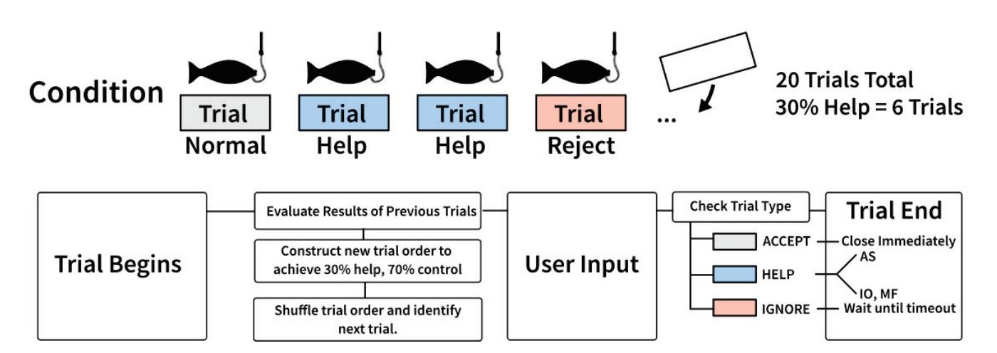
**Figure 3.** Each condition consisted of 20 trials. In the helped conditions, help trials with predefined outcomes (blue) were shuffled with normal (no PAM) trials (gray) to provide users with 30% help. Forced rejections (red) were inserted when people were succeeding above the 70% target control rate.
#### 2.4. Experimental Setup
Initially, the cap was mounted on the participants and the signal quality was checked to make sure there was good signal quality (see Figure 4). In the calibration session, the participants were asked to perform MI 30 times. They were instructed to perform kinesthetic or first-person MI by recalling the sensation of doing a palmar grasp of the right hand. They were asked to maintain the imaginary contraction for four seconds while avoiding blinking or making contractions of facial muscles or other muscles. A visual cue of a red arrow pointing to the right was shown to the participants for four seconds to indicate when to start and stop the imaginary contraction. Thirty trials of idle activity were also recorded when the participants were resting, a visual cue with the text "Rest" was displayed to the participants for four seconds. Each MI trial was followed by an idle activity trial. After the BCI was calibrated the experiment started. The experiment followed a within-subject design, where participants played four conditions each (a control condition without PAM, and one condition per PAM). To avoid any order bias, we used a Latin square design for PAM conditions. The participants were introduced to one condition at a time. Prior to each condition, the facilitator introduced the condition by explaining the PAM.
- Control condition: The facilitator explained the core game. This condition was always the first condition the participants went through.
- Augmented Success: "*In this condition, the fisherman will occasionally become stronger.*"
- Mitigated Failure: "*In this condition, occasionally a clip on the fishing rod will prevent the fish from escaping.*"
- Input Override: "*In this condition, a girl will occasionally come to help you.*"
In each condition, the participants played for 20 trials and tried to catch as many fish as possible. For the final fish in each condition, if the participants had no more trials left, the fish would escape.
91
*Sensors* **2022**, *22*, 9051
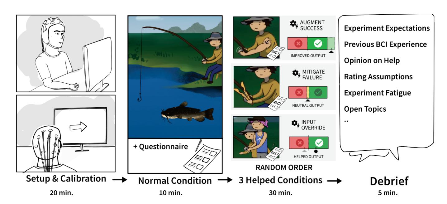
**Figure 4.** Each participant in the experiment (1) underwent BCI setup and BCI calibration, (2) played a fishing game in four conditions, starting with the normal condition, followed by (3) three helped conditions in a shuffled order. Participants were then debriefed about their experiences.
In accordance with previous BCI-related studies, we focused on the user experience [34–37], and the dependent variables we measured were frustration and perceived control. After each condition, participants rated on a Likert scale their perceived control ("*I felt I was in control of the fisherman reeling in the fish.*") 1 (Strongly disagree) to 7 (Strongly agree) and frustration ("*How much frustration did you feel in this condition?*") from 1 (Strongly absent) to 7 (Strongly pronounced). They were informed to do this while considering the condition as a whole ("*Please rate your experience as a whole during this play-through.*"). The participants were kept unaware of their actual BCI performances from their calibration and test sessions so that they would not influence their ratings.
At the end of the experiment, the participants were debriefed. First, participants were inquired as to their prior expectations of the experiment, for instance, whether they thought they would do better or worse, and how it was to control the BCI. Participants elaborated on any previous experience with BCI, to allow for grouping and rating difference checks in the analysis. Participants pointed out the hardest and easiest condition, and what their thoughts were on the PAMs. We went through their Likert scale ratings with them, to check for potential misunderstandings, i.e., prompting them to explain extreme values, which were used in the qualitative analysis to reason about outlier data points.
#### 2.5. Data Analysis
#### 2.5.1. Variables
The study collected continuous data and MI detections from the BCI and event data from the game (e.g., user input and game activity). An overview of the variable pool can be found in Table 2. Each participant contributed perceived control and frustration Likert scale item scores for each of the four conditions, which was merged with the game data and analyzed in R studio. Individual conditions were reviewed to identify potential abnormalities. From the combined dataset, we selected eight variables (MI conversion rate, PAM rate, condition, positive feedback, fish caught, fish lost, fish reel, and fish unreel) to evaluate people's ratings of perceived control and frustration. Fish unreel, fish reel, fish lost, and fish caught were included in the analysis because they represent the types of positive and negative feedback presented in the game. PAM Rate was included to analyze the impact of introducing help. In addition, we included the condition variable to analyze for differences between three types of help (augmented success, mitigated failure, and input override) and the normal condition. MI conversion rate was included to compare how users' ability to perform MI to obtain successful trials affected perceived control and frustration ratings.
92
*Sensors* **2022**, *22*, 9051
**Table 1.** Trials were manipulated by the urn model to target 30% help and limit control in help conditions. The table shows the mean % of how help conditions changed the outcomes as described in Section 2.3.1, compared to the normal condition (reference condition).
| Augmented Success (AS) | | Input Override (IO) | | Mitigated Failure (MF) | | Normal Condition | |
|---------------------------------|-----|---------------------------|-----|--------------------------|-----|----------------------|-----|
| Negative (No Change) | 46% | Negative (No Change) | 33% | Negative (No Change) | 30% | Negative (No Change) | 42% |
| Positive (No Change) | 28% | Negative to Positive (IO) | 15% | Negative to Neutral (MF) | 17% | Positive (No Change) | 57% |
| Positive to Extra Positive (AS) | 14% | Positive (No Change) | 37% | Positive (No Change) | 40% | | |
| Positive to Negative | 12% | Positive to Positive (IO) | 15% | Positive to Neutral (MF) | 13% | | |
**Table 2.** Descriptions of dependent (response) and independent (explanatory) variables used in the analysis and their minimum (Min) and maximum values (Max), means, and standard deviation(s) (SD).
| Variables | Min | Max | Mean | SD | Description |
|-------------------|-----|-----|------|------|-----------------------------------------------------------------------------------------------------------------------------------------------------|
| Response | | | | | |
| Perceived Control | 0 | 1 | 0.46 | 0.27 | Normalized 7-point Likert scale rating by participants after playing a condition. |
| Frustration | 0 | 1 | 0.50 | 0.29 | Normalized 7-point Likert scale rating by participants after playing a condition. |
| Explanatory | | | | | |
| MI Conv. Rate | 0 | 1 | 0.54 | 0.28 | Normalized count of trials that were caused by successful motor imagery activations in a condition. |
| Pos. Feedback | 0 | 1 | 0.52 | 0.24 | Normalized count of how many trials delivered a positive outcome (reeling fish, catching fish, receiving help) in a condition, regardless of cause. |
| Fish Caught | 0 | 8 | 3.59 | 2.39 | Count of how many fish were reeled all the way up and caught in a given condition. |
| Fish Lost | 0 | 6 | 1.69 | 1.69 | Count of how many fish participants lost when playing a given condition. |
| Fish Reel | 0 | 20 | 6.75 | 3.54 | Count of how many times participants managed to reel a fish closer to them in a condition. |
| Fish Unreel | 0 | 14 | 6.54 | 3.31 | Count of how many times the fishing rod unreeled (the fish trying to escape) in a condition. |
| PAM rate | 0 | 0.3 | 0.18 | 0.13 | Normalized count of trials in which participants received help in a condition. |
| Condition | - | - | - | - | Participants played four conditions: Normal (no PAM), augmented success, input override, and mitigated failure. |
#### 2.5.2. Analysis Method
Many of the explanatory variables represent different ways to consider positive feedback and it is not clear which variables are better at explaining how people rate perceived control and frustration. To investigate this question, we constructed models from the variables and tested whether models, which included a variable, were significantly different to a null model without the variable present. We used cumulative link mixed models from the ordinal package [50] fitted with Laplace approximation, also known as an ordered response mixed model. We used cumulative link mixed models in our analysis because they provide a regression framework that treats observations made in the experiment's response variables frustration and perceived control correctly as ordinal data. To counter potential pseudoreplication [51] from our repeated measures design, we used *Participant* as the basis for the null model and modeled it as random intercepts to account for by-subject baseline rating differences. We determined the most suitable model from our variables by using forward step-wise selection, which added variables based on the Akaike information criterion (AIC). We tested for significant predictors of frustration and perceived control, using Likelihood ratio tests with a *p*-value threshold of 0.05. The variables were tested as fixed effects and determined based on their known relationship in affecting control or positive feedback in the experiment.
93
*Sensors* **2022**, *22*, 9051
Participant Likert scores of perceived control and frustration were summarized visually through to aid exploratory analysis. In contrast to the cumulative link mixed models, participants' Likert scores were normalized from 1–7 to 0–1, treated numerically in tables, and visualized with linear regression for exploratory analysis.
Qualitative data included participant video recordings, game recordings, and notes taken during debriefing interviews, which we thematically analyzed for repeated patterns [52]. Due to a mistake in the experimental procedure, Participant 2 had missing data and was, therefore, excluded from the analysis.
#### 3. Results
Eighteen participants played and scored four conditions, shown in Table 3. In three conditions, an urn model manipulated their experience, as summarized in Table 1.
**Table 3.** Participant demographics, individual scores per condition (Likert scales of perceived control and frustration), MI conversion rate (% of MI events, which resulted in positive outcomes), and positive feedback (% of trials, which delivered positive feedback). Gray denotes high frustration, low perceived control, low MI conversion rate, or low positive feedback.
| Variable | 1 | 3 | 4 | 5 | 6 | 7 | 8 | 9 | 10 | 11 | 12 | 13 | 14 | 15 | 16 | 17 | 18 | 19 |
|-----------------------|------|------|------|------|------|------|------|------|------|-------|------|------|------|------|------|------|------|------|
| Gender | F | M | M | M | M | F | M | M | F | F | F | F | M | M | M | M | M | F |
| Age | 27 | 29 | 60 | 27 | 22 | 23 | 24 | 24 | 23 | 22 | 33 | 24 | 22 | 24 | 21 | 28 | 26 | 25 |
| Perceived Performance | 0.85 | 0.95 | 0.35 | NA | 0.7 | 0.75 | 0.2 | 0.75 | 0.8 | 0.075 | 0.6 | 0.5 | 0.15 | 0.35 | 0.6 | 0.35 | 0.45 | 0.5 |
| BCI Experience | Yes | Yes | No | No | Yes | Yes | Yes | Yes | Yes | Yes | No | No | Yes | No | No | No | Yes | Yes |
| Perc. Control | 0.67 | 0.75 | 0.21 | 0.37 | 0.63 | 0.58 | 0.29 | 0.54 | 0.46 | 0.04 | 0.29 | 0.71 | 0.11 | 0.54 | 0.75 | 0.42 | 0.38 | 0.54 |
| Frustration | 0.33 | 0.13 | 1.00 | 0.38 | 0.54 | 0.42 | 0.50 | 0.58 | 0.42 | 1.00 | 0.54 | 0.25 | 0.67 | 0.50 | 0.29 | 0.83 | 0.54 | 0.21 |
| MI Conv. Rate | 92% | 85% | 21% | 61% | 32% | 80% | 32% | 75% | 36% | 11% | 71% | 80% | 27% | 52% | 34% | 45% | 78% | 55% |
| Pos. Feedback | 78% | 74% | 28% | 57% | 35% | 70% | 35% | 68% | 40% | 18% | 66% | 70% | 32% | 50% | 40% | 49% | 65% | 52% |
| Aug. Success | | | | | | | | | | | | | | | | | | |
| Perc. Control | 0.67 | 0.83 | 0.33 | 0.33 | 0.50 | 0.33 | 0.33 | 0.17 | 0.33 | 0.00 | 0.17 | 0.50 | 0.33 | 0.67 | 1.00 | 0.67 | 0.17 | 0.67 |
| Frustration | 0.33 | 0.17 | 1.00 | 0.17 | 0.67 | 0.50 | 0.67 | 0.83 | 0.33 | 1.00 | 0.50 | 0.17 | 0.67 | 0.33 | 0.17 | 0.67 | 0.67 | 0.17 |
| MI Conv. Rate | 95% | 80% | 15% | 60% | 15% | 90% | 50% | 30% | 35% | 15% | 85% | 75% | 35% | 65% | 45% | 45% | 85% | 55% |
| Pos. Feedback | 65% | 60% | 15% | 50% | 15% | 55% | 35% | 20% | 25% | 15% | 70% | 50% | 30% | 50% | 45% | 45% | 60% | 45% |
| Fish Caught | 0 | 6 | 1 | 4 | 1 | 5 | 1 | 0 | 2 | 1 | 8 | 4 | 2 | 6 | 5 | 6 | 5 | 5 |
| Fish Lost | 0 | 0 | 5 | 1 | 5 | 2 | 4 | 5 | 4 | 5 | 0 | 2 | 3 | 2 | 3 | 2 | 2 | 2 |
| Input Override | | | | | | | | | | | | | | | | | | |
| Perc. Control | 0.50 | 0.50 | 0.17 | 0.50 | 0.67 | 0.67 | 0.33 | 0.50 | 0.50 | 0.00 | 0.33 | 0.67 | 0.00 | 0.67 | 0.83 | 0.33 | 0.33 | 0.33 |
| Frustration | 0.50 | 0.17 | 1.00 | 0.50 | 0.67 | 0.50 | 0.33 | 0.50 | 0.17 | 1.00 | 0.67 | 0.83 | 0.50 | 0.50 | 0.33 | 0.83 | 0.50 | 0.50 |
| MI Conv. Rate | 100% | 95% | 5% | 55% | 35% | 95% | 30% | 95% | 15% | 5% | 50% | 90% | 30% | 65% | 40% | 30% | 65% | 45% |
| Pos. Feedback | 100% | 95% | 35% | 70% | 50% | 100% | 55% | 95% | 40% | 35% | 60% | 95% | 50% | 75% | 65% | 60% | 70% | 60% |
| Fish Caught | 0 | 8 | 2 | 6 | 3 | 7 | 5 | 8 | 2 | 2 | 4 | 7 | 3 | 7 | 4 | 4 | 5 | 4 |
| Fish Lost | 0 | 0 | 3 | 0 | 2 | 0 | 2 | 0 | 3 | 4 | 1 | 0 | 2 | 0 | 1 | 1 | 0 | 2 |
| Mit. Failure | | | | | | | | | | | | | | | | | | |
| Perc. Control | 0.50 | 0.67 | 0.00 | 0.33 | 0.67 | 0.33 | 0.33 | 0.67 | 0.33 | 0.17 | 0.00 | 0.67 | | 0.50 | 0.67 | 0.17 | 0.33 | 0.67 |
| Frustration | 0.33 | 0.17 | 1.00 | 0.33 | 0.33 | 0.50 | 0.33 | 0.67 | 0.50 | 1.00 | 0.83 | 0.00 | | 0.50 | 0.33 | 1.00 | 0.50 | 0.00 |
| MI Conv. Rate | 90% | 80% | 10% | 70% | 30% | 50% | 25% | 75% | 30% | 25% | 80% | 75% | | 55% | 15% | 40% | 85% | 60% |
| Pos. Feedback | 60% | 55% | 5% | 50% | 25% | 40% | 25% | 55% | 30% | 20% | 65% | 55% | | 50% | 15% | 25% | 55% | 45% |
| Fish Caught | 0 | 4 | 0 | 4 | 1 | 2 | 1 | 5 | 1 | 1 | 5 | 4 | | 3 | 1 | 1 | 4 | 3 |
| Fish Lost | 0 | 0 | 4 | 1 | 2 | 1 | 3 | 0 | 2 | 3 | 0 | 0 | | 1 | 3 | 2 | 0 | 1 |
| Ref. Condition | | | | | | | | | | | | | | | | | | |
| Perc. Control | 1.00 | 1.00 | 0.33 | 0.33 | 0.67 | 1.00 | 0.17 | 0.83 | 0.67 | 0.00 | 0.67 | 1.00 | 0.00 | 0.33 | 0.50 | 0.50 | 0.67 | 0.50 |
| Frustration | 0.17 | 0.00 | 1.00 | 0.50 | 0.50 | 0.17 | 0.67 | 0.33 | 0.67 | 1.00 | 0.17 | 0.00 | 0.83 | 0.67 | 0.33 | 0.83 | 0.50 | 0.17 |
| MI Conv. Rate | 85% | 85% | 55% | 60% | 50% | 85% | 25% | 100% | 65% | 0% | 70% | 80% | 15% | 25% | 35% | 65% | 75% | 60% |
| Pos. Feedback | 85% | 85% | 55% | 60% | 50% | 85% | 25% | 100% | 65% | 0% | 70% | 80% | 15% | 25% | 35% | 65% | 75% | 60% |
| Fish Caught | 0 | 6 | 3 | 5 | 4 | 8 | 1 | 8 | 4 | 0 | 6 | 6 | 1 | 2 | 2 | 5 | 7 | 4 |
| Fish Lost | 0 | 0 | 2 | 1 | 2 | 0 | 4 | 0 | 0 | 6 | 0 | 0 | 5 | 4 | 3 | 0 | 0 | 2 |
94
*Sensors* **2022**, *22*, 9051
#### 3.1. Perceived Control
Forward stepwise selection constructed nine significant models for perceived control, listed at the top of Table 4. Six of eight explanatory variables resulted in significant models, where *Fish Lost* performed best in terms of AIC, ML, and LR when compared to the null model. *Fish Lost* was, therefore, chosen as the null model, and to form the basis for the model construction in the forward stepwise selection, to see if the variable could be combined with others. Three of the eight fixed effects (*Fish Caught*, *Condition*, and *PAM Rate*) made significant improvements to the model with *Fish Lost*. Examination of the *Fish Lost* + *PAM Rate* model resulted in the model outcomes shown at the bottom of Table 4. Contrary to expectations, *PAM Rate* was estimated to negatively affect participants' rating of perceived control (estimate = −7.86, *p* < 0.001)—when people received more help, their ratings generally were lower. The examination of the second-best model *Fish Lost + Condition* estimated that the negative effect came from the conditions *input override* and (estimate = −2.04, *p* = 0.004) *mitigated failure* (estimate = −2.08, *p* = 0.004), while *augmented success*'s estimate was marginally positive it did not significantly affect perceived control (Estimate = 0.2, *p* = 0.786). The negative effects of input override and mitigated failure are also evident in the top row of Figure 5, which visualizes the relationship between positive feedback and perceived control in each condition. From the visual inspection, we observed that when participants experienced more than 50% of positive feedback, they tended to favor conditions without help. Only in cases where positive feedback was low (less than 50%), did participants rate help higher in the augmented success condition.
**Table 4.** (Top) Results of significant likelihood ratio tests predicting perceived control, with the AIC (Akaike information criterion), ML (maximum likelihood), LR (likelihood ratio), and *χ*2 (significance). (Bottom) fixed effect estimates for predicting perceived control in the best model "Fish Lost + PAM Rate".
| Predicted | Fixed Effect | AIC | ML | LR | χ² |
|-------------------|-------------------------|----------|------------|---------|--------|
| Perceived Control | Fish Lost + PAM Rate | 215.82 | -98.91 | 15.61 | <0.001 |
| | Fish Lost + Condition | 219.11 | -98.55 | 16.32 | 0.001 |
| | Fish Lost + Fish Caught | 226.70 | -104.35 | 4.72 | 0.030 |
| | Fish Lost | 229.43 | -106.71 | 24.05 | <0.001 |
| | Fish Caught | 232.12 | -108.06 | 21.36 | <0.001 |
| | Pos. Feedback | 233.27 | -108.63 | 20.21 | <0.001 |
| | MI Conv. Rate | 237.67 | -110.83 | 15.81 | <0.001 |
| | Fish Reel | 242.10 | -113.05 | 11.38 | 0.001 |
| | Fish Unreel | 245.62 | -114.81 | 7.86 | 0.005 |
| Predicted | Fixed Effect | Estimate | Std. Error | z Value | p |
| Perceived Control | PAM Rate | -7.86 | 2.14 | -3.68 | <0.001 |
| | Fish Lost | -1.39 | 0.27 | -5.11 | <0.001 |
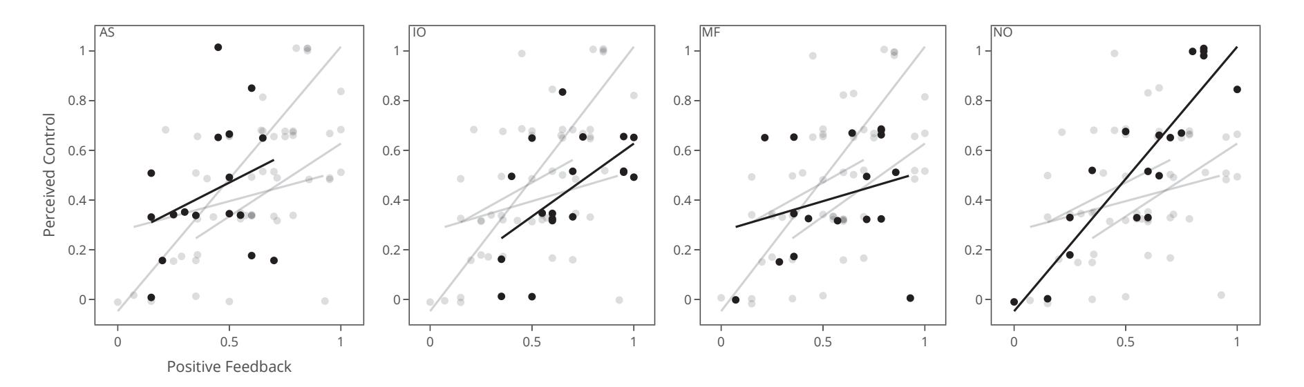
**Figure 5.** *Cont*.
95
*Sensors* **2022**, *22*, 9051
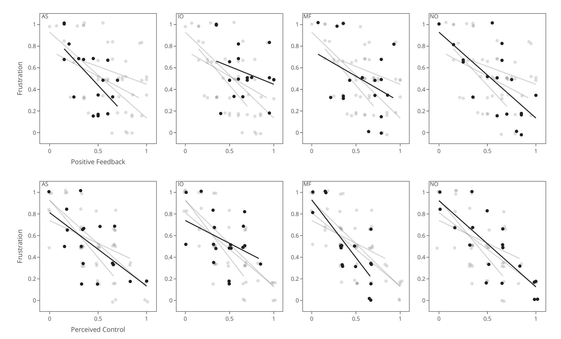
**Figure 5.** The relationship between perceived control and positive feedback is shown in the top row of each of the four conditions, while the relationship between frustration and positive feedback is shown in the middle row. In the bottom row, the relationship between frustration and perceived control is shown. AS: augmented success, IO: input override, MF: mitigated failure, and NO: normal condition without PAM help. Each data point represents the rating of a single participant.
#### 3.2. Frustration
Forward stepwise selection constructed four significant models, using four of the eight explanatory variables to predict frustration, listed at the top of Table 5. Escaping fish frustrated the participants (*Fish Lost*, Estimate = 0.62, *p* = 0.003), and conversely, participants were less frustrated when they caught more fish (*fish caught*, estimate = −0.39, *p* < 0.001). However, participants' frustration ratings were not affected by the type of help they received. For frustration, no models that included *PAM Rate* or *Condition* were different from the null model. Visual inspections of the middle row plots in Figure 5 show a clear downward relationship between frustration ratings and positive feedback for all conditions. Augmented success and normal conditions showed similar relationships while the input override showed overall higher frustration ratings despite participants receiving more positive feedback than any other condition on average (M = 0.67, SD = 0.22). Input override and mitigated failure both showed less decreasing changes in the frustration ratings as positive feedback increased, indicating that higher control did not make as much of a difference in people's frustrations. When plotting frustration and perceived control were against each other (Figure 5, bottom row), a clear correlation was shown in all conditions with the exception of input override.
The MI conversion rate was a significant fixed effect in models of perceived control and frustration, but variables relating to in-game feedback (fish lost, fish caught) resulted in models with lower AIC, and lower ML (shown in Tables 4 and 5). Participants had widely different MI conversion rates between 5–100% (M = 0.54, SD = 0.28).
96
*Sensors* **2022**, *22*, 9051
**Table 5.** (Top) Results of significant likelihood ratio tests predicting frustration. (Bottom) fixed effect estimates for predicting frustration in the best model "Fish Lost".
| Predicted | Fixed Effect | AIC | ML | LR | χ² |
|-------------|---------------|--------|---------|------|-------|
| Frustration | Fish Lost | 239.63 | −111.82 | 8.81 | 0.003 |
| | Fish Caught | 240.46 | −112.23 | 7.99 | 0.005 |
| | MI Conv. Rate | 242.49 | −113.25 | 5.95 | 0.015 |
| | Pos. Feedback | 244.20 | −114.10 | 4.24 | 0.039 |
#### 3.3. Qualitative Results
Playing the control condition, several participants (10/19) found it easy to control, while a few participants (3/19) said they were learning the game in this condition, which reduced the frustration of a few participants (2/19). The in-game character taking over the fishing rod in the input override condition was frustrating for most participants (13/19), because they wanted to solve the task themselves: "*I did not want any help from the girl.*" (P7, 11, 17). Input override removed their agency "*it doesn't really feel like my attempt when someone else was helping.*" (P2), and reduced the legitimacy of the reward "*it was less rewarding [to catch the fish] because I got help from the girl.*" (P14, 16). The mitigated failure condition highlighted participants' failures, as they had another try but frustrated only very few (3/19). However, few participants (4/19) found the extra try less frustrating, "*the clip [mitigated failure] was encouraging because you got a second try.*" (P2). Some participants (6/19) found augmented success easy to control, as one participant mentioned that the condition felt less patronizing than the rest. Catching a fish made some participants (7/19) feel in control of the fisherman reeling in the fish. Not being able to decide when to trigger the PAMs in the three conditions caused confusion for some participants (5/19). Not being able to trigger the last action causing the fish to escape frustrated a few participants (4/19). Losing control caused a few participants (2/19) to feel frustration. P11 felt they had no control despite having good calibration.
#### 4. Discussion
In this study, three PAMs (augmented success, mitigated failure, and input override) were implemented in an online MI-BCI to evaluate their effects on perceived control and frustration. The help from PAMs was perceived differently, but generally, input override frustrated participants the most since they wanted to perform the tasks by themselves, or they blamed themselves for not succeeding since they knew they were unable to trigger the BCI when they received help despite its positive outcome. Moreover, in the mitigated failure condition, a similar tendency in frustration ratings was seen since the participants were aware when they were unable to trigger the BCI, although neutral feedback was provided and that could have caused the participants to blame themselves. Both PAMs reduced the participants perceived control. The augmented success did not increase frustration or reduce perceived control. It should be noted that the participants were explicitly informed about the PAMs before they tried the conditions, so it is possible that the PAMs could be perceived differently by naive players.
Participants with lower BCI control generally rated their perceived control higher in the PAM conditions with respect to the normal condition without PAM and vice versa for participants with better BCI control. The lower ratings of perceived control for the participants with better BCI performance could be partly explained by the fact that their BCI performance could be slightly impeded in the PAM conditions. However, the participants were kept unaware of their actual BCI performance, so they could not be sure about the potential reduction of their BCI performance in the PAM conditions. They only had their own experience to judge from. Perceived control negatively correlated with frustration in all conditions, but with a weaker correlation for the input override PAM, which frustrated the participants the most. The negative correlation between perceived control and frustra97
*Sensors* **2022**, *22*, 9051
tion is in agreement with our previous findings [34,35]. The findings regarding positive feedback as a predictor of perceived control and frustration agree with a similar study using online MI-BCI methodology with fabricated input [35]. Surrogate BCI studies have also reported that higher levels of positive feedback increase perceived control and reduce frustration [34,36,37]. Perceived control was rated differently in the PAM conditions for participants with the lowest and highest BCI performance. A similar finding was reported for BCI control with biased feedback, where users with poor BCI performances benefited from biased feedback and users with good BCI performances were impeded by this [53]. It should be noted that in the current study the BCI performance was fairly low with few participants achieving BCI performances higher than 80%. Thus, the entire spectrum of the BCI performance has not been covered sufficiently and, hence, it is unknown if similar ratings of perceived control in PAM conditions are applicable for BCI performances higher than 80%. The negative correlation between perceived control and frustration in all conditions was expected since it was shown that perceived control and frustration are inversely correlated in both able-bodied users and people with a stroke [34,35]. However, in the input override condition, a weaker negative correlation was found. This could be due to the fact that explicit help overruled the actual control and, hence, reduced the perceived control and increased frustration, which was also indicated by several participants in the qualitative analysis. Input override is similar to positive fabricated input, which has previously been shown to lead to a correlation between perceived control and frustration [35], but the difference in the current study is that input override is not concealed in the game, and the participants were informed about the input override PAM prior to the condition. Thus, it should be considered if input override should be concealed instead of being explicitly articulated in the interaction, which may reduce the frustration.
#### 4.1. Methodological Considerations
As outlined, the BCI performance in this study was modest and did not cover the higher end of the spectrum. This does not necessarily mean that the participants were poor BCI performers but the design of the interaction with only a two-second input window might have been too challenging. The participants only had two seconds to produce MI, contrary to our previous study, which allowed for MI during a five-second window, which yielded a better BCI performance with recognition rates exceeding 90%. The BCI setup, hardware, and processing were identical to our previous study [35]. In hindsight, two seconds may be too little time to perform MI (or to perform more than one attempt during an input window), especially when the participants had to produce MI exceeding a specific threshold for 0.5 consecutive seconds. In future studies, we would recommend increasing the duration of the input window up to five seconds. This would increase the likelihood of a false positive detection being counted as a true positive since a longer input window means that more false positive detections can occur [12]. This risk, however, could be reduced by setting a higher threshold that has to be exceeded for a given period of time. The threshold should be set such that the number of false positive detections is minimized but that it is still possible for the user to activate the BCI. In some applications/interactions, it could be desirable to set the threshold such that either more or fewer true and false positives are accepted. In applications requiring higher thresholds, i.e., a lower number of true and false positives, PAMs may be more useful since there is more room to help the user on the contrary to applications with lower thresholds, where a higher number of true and false positives lead to many successful trials potentially making the PAMs redundant. Lastly, the BCI performance can be enhanced using other signal processing and classification methods or training the user in performing MI.
In the current study, healthy users participated, but the intended use of a gamified MI-BCI system is for stroke rehabilitation. The findings in the current study cannot be directly transferred to a population of stroke patients, which, besides motor impairments, may have cognitive impairments and different levels of technological prerequisites. Stroke
98
*Sensors* **2022**, *22*, 9051
patients are generally above 60 years of age, while the participants in the current study consisted of able-bodied primarily in their twenties.
#### 4.2. Implications
In this study, we showed that it was possible to integrate different PAMs in a BCI paradigm that are usable and meaningful for stroke rehabilitation. The PAMs created different reactions from the users, which could be useful for designing engaging games. The findings though suggest that the use of explicit input overrides should be considered carefully to avoid frustration, but it may still be useful to use it to create engaging interactions for the user and stroke patients may perceive help differently than the able-bodied participants in this study. Augmented success can be used to highlight the successes of the users, which could strengthen motivation. By using multiple PAMs, different types of games with various designs can be created, which could support the rehabilitation efforts to get the patient to train more.
Moreover, PAMs could potentially be used in training sessions to learn to perform MI. For this application though, it is expected that augmented success and mitigated failure would be the best choices since input override will provide inaccurate feedback to the user while augmented success could reinforce the learning and mitigated failure would not discourage users.
#### 4.3. Future Perspectives
In future studies where the entire performance spectra need to be covered in systematic ways, researchers could consider using surrogate BCIs that share the same characteristics as an online MI-BCI but with other more reliable input methods, such as a concealed eyetracker (an EEG cap can be mounted and it can be conveyed to the users that blink, as picked up by the BCI) [34,35]. In this way, there is access to the ground truth and performance can be artificially controlled, such that users experience different levels of control that can be similar across the study population. As outlined previously, stroke patients differ from the participants included in the current study, and it is important to learn how stroke patients react to different PAMs, so they can be used in the best way for engaging interactions in rehabilitation. Another aspect that should be tested, is how users react to PAMs when they attend multiple training sessions. It is expected that the BCI performance could improve as a result of training and familiarization with the BCI system and interaction. In the current work, PAMs were rated differently for better-performing users compared to users with lower BCI performance. Lastly, the type of interaction should be considered if the feedback should be realistic, e.g., using a humanoid hand or if the feedback can be more abstract [48]. The former is shown to improve the ownership and perceived control over more abstract feedback, but the latter could result in more engaging or fun interactions by providing the designers of rehabilitation games with more artistic freedom.
#### 5. Conclusions
This study showed that PAMs could be integrated into an online BCI based on MI, and the different PAMs could assist the participants. The amount of combined positive feedback received from regular and PAM-enhanced inputs could explain the perceived control and frustration of participants. The different PAMs can be used in a more varied and richer way to aid users with poor BCI performance beyond adding simple extra positive sham feedback. The condition that explicitly depicted input override frustrated participants the most, but it is clear that people have different preferences in how they can be helped. Within the different types of PAMs, game developers can exercise tremendous artistic freedom to create engaging interactions for BCI training that either directly manipulate the outcomes of a single action or its effect in a bigger task context.
99
*Sensors* **2022**, *22*, 9051
**Author Contributions:** Conceptualization, M.J., B.I.H. and H.K.; methodology, M.J., B.I.H., M.S.K. and H.K.; software, M.J. and B.I.H.; validation, B.I.H. and M.S.K.; formal analysis, B.I.H.; investigation, B.I.H. and M.S.K.; resources, M.J.; data curation, B.I.H. and M.S.K.; writing—original draft preparation, M.J. and B.I.H.; writing—review and editing, M.J., B.I.H., M.S.K. and H.K.; visualization, B.I.H.; supervision, M.J. and H.K.; project administration, B.I.H.; funding acquisition, M.J. All authors have read and agreed to the published version of the manuscript.
**Funding:** This research was funded by VELUX FONDEN grant number 22357.
**Institutional Review Board Statement:** The study was conducted in accordance with the Declaration of Helsinki, and approved by the North Denmark Region Committee on Health Research Ethics (N-20130081).
**Informed Consent Statement:** Informed consent was obtained from all subjects involved in the study.
**Data Availability Statement:** The data that support the findings of this study are available upon reasonable request from the corresponding author.
**Acknowledgments:** The authors would like to thank Ingeborg G. Rossau, Mozes Adorjan Miko, Jedrzej Jacek Czapla, and Rasmus Bugge Skammelsen for the development of the game-based interaction, and Dávid Gulyás, Thomas Kjeldsen, and Steffen Lehmann for assistance during the data collection.
**Conflicts of Interest:** The authors declare no conflict of interest. The funders had no role in the design of the study; in the collection, analyses, or interpretation of data; in the writing of the manuscript; or in the decision to publish the results.
#### References
- 1. Feigin, V.L.; Forouzanfar, M.H.; Krishnamurthi, R.; Mensah, G.A.; Connor, M.; Bennett, D.A.; Moran, A.E.; Sacco, R.L.; Anderson, L.; Truelsen, T.; et al. Global and regional burden of stroke during 1990–2010: Findings from the Global Burden of Disease Study 2010. *Lancet* **2014**, *383*, 245–254. [CrossRef]
- 2. Langhorne, P.; Coupar, F.; Pollock, A. Motor recovery after stroke: A systematic review. *Lancet Neurol.* **2009**, *8*, 741–754. [CrossRef]
- 3. Krakauer, J.W. Motor learning: Its relevance to stroke recovery and neurorehabilitation. *Curr. Opin. Neurol.* **2006**, *19*, 84–90. [CrossRef] [PubMed]
- 4. Belda-Lois, J.M.; Mena-del Horno, S.; Bermejo-Bosch, I.; Moreno, J.C.; Pons, J.L.; Farina, D.; Iosa, M.; Molinari, M.; Tamburella, F.; Ramos, A.; et al. Rehabilitation of gait after stroke: A review towards a top-down approach. *J. Neuroeng. Rehabil.* **2011**, *8*, 66. [CrossRef]
- 5. Dimyan, M.A.; Cohen, L.G. Neuroplasticity in the context of motor rehabilitation after stroke. *Nat. Rev. Neurol.* **2011**, *7*, 76–85. [CrossRef] [PubMed]
- 6. Biasiucci, A.; Leeb, R.; Iturrate, I.; Perdikis, S.; Al-Khodairy, A.; Corbet, T.; Schnider, A.; Schmidlin, T.; Zhang, H.; Bassolino, M.; et al. Brain-actuated functional electrical stimulation elicits lasting arm motor recovery after stroke. *Nat. Commun.* **2018**, *9*, 2421. [CrossRef]
- 7. Pichiorri, F.; Morone, G.; Petti, M.; Toppi, J.; Pisotta, I.; Molinari, M.; Paolucci, S.; Inghilleri, M.; Astolfi, L.; Cincotti, F.; et al. Brain–computer interface boosts motor imagery practice during stroke recovery. *Ann. Neurol.* **2015**, *77*, 851–865. [CrossRef]
- 8. Grosse-Wentrup, M.; Mattia, D.; Oweiss, K. Using brain–computer interfaces to induce neural plasticity and restore function. *J. Neural Eng.* **2011**, *8*, 025004. [CrossRef]
- 9. Niazi, I.K.; Mrachacz-Kersting, N.; Jiang, N.; Dremstrup, K.; Farina, D. Peripheral electrical stimulation triggered by self-paced detection of motor intention enhances motor evoked potentials. *IEEE Trans. Neural Syst. Rehabil. Eng.* **2012**, *20*, 595–604. [CrossRef]
- 10. Jochumsen, M.; Navid, M.S.; Nedergaard, R.W.; Signal, N.; Rashid, U.; Hassan, A.; Haavik, H.; Taylor, D.; Niazi, I.K. Self-paced online vs. cue-based offline brain–computer interfaces for inducing neural plasticity. *Brain Sci.* **2019**, *9*, 127. [CrossRef]
- 11. Jochumsen, M.; Navid, M.S.; Rashid, U.; Haavik, H.; Niazi, I.K. EMG-versus EEG-triggered electrical stimulation for inducing corticospinal plasticity. *IEEE Trans. Neural Syst. Rehabil. Eng.* **2019**, *27*, 1901–1908. [CrossRef] [PubMed]
- 12. Niazi, I.K.; Navid, M.S.; Rashid, U.; Amjad, I.; Olsen, S.; Haavik, H.; Alder, G.; Kumari, N.; Signal, N.; Taylor, D.; et al. Associative cued asynchronous BCI induces cortical plasticity in stroke patients. *Ann. Clin. Transl. Neurol.* **2022**, *9*, 722–733. [CrossRef] [PubMed]
- 13. Jochumsen, M.; Cremoux, S.; Robinault, L.; Lauber, J.; Arceo, J.C.; Navid, M.S.; Nedergaard, R.W.; Rashid, U.; Haavik, H.; Niazi, I.K. Investigation of optimal afferent feedback modality for inducing neural plasticity with a self-paced brain-computer interface. *Sensors* **2018**, *18*, 3761. [CrossRef] [PubMed]
- 14. Xu, R.; Jiang, N.; Mrachacz-Kersting, N.; Lin, C.; Prieto, G.A.; Moreno, J.C.; Pons, J.L.; Dremstrup, K.; Farina, D. A closed-loop brain–computer interface triggering an active ankle–foot orthosis for inducing cortical neural plasticity. *IEEE Trans. Biomed. Eng.* **2014**, *61*, 2092–2101.
100
*Sensors* **2022**, *22*, 9051
- 15. Jochumsen, M.; Janjua, T.A.M.; Arceo, J.C.; Lauber, J.; Buessinger, E.S.; Kæseler, R.L. Induction of neural plasticity using a low-cost open source brain-computer interface and a 3D-printed wrist exoskeleton. *Sensors* **2021**, *21*, 572. [CrossRef] [PubMed]
- 16. De Vries, S.; Mulder, T. Motor imagery and stroke rehabilitation: A critical discussion. *J. Rehabil. Med.* **2007**, *39*, 5–13. [CrossRef]
- 17. Cervera, M.A.; Soekadar, S.R.; Ushiba, J.; Millán, J.d.R.; Liu, M.; Birbaumer, N.; Garipelli, G. Brain-computer interfaces for post-stroke motor rehabilitation: A meta-analysis. *Ann. Clin. Transl. Neurol.* **2018**, *5*, 651–663. [CrossRef]
- 18. Nojima, I.; Sugata, H.; Takeuchi, H.; Mima, T. Brain–Computer Interface Training Based on Brain Activity Can Induce Motor Recovery in Patients with Stroke: A Meta-Analysis. *Neurorehabilit. Neural Repair* **2021**, *36*, 83–96. [CrossRef] [PubMed]
- 19. Kenah, K.; Bernhardt, J.; Cumming, T.; Spratt, N.; Luker, J.; Janssen, H. Boredom in patients with acquired brain injuries during inpatient rehabilitation: A scoping review. *Disabil. Rehabil.* **2018**, *40*, 2713–2722. [CrossRef]
- 20. de Castro-Cros, M.; Sebastian-Romagosa, M.; Rodríguez-Serrano, J.; Opisso, E.; Ochoa, M.; Ortner, R.; Guger, C.; Tost, D. Effects of gamification in BCI functional rehabilitation. *Front. Neurosci.* **2020**, *14*, 882. [CrossRef]
- 21. Mubin, O.; Alnajjar, F.; Jishtu, N.; Alsinglawi, B.; Al Mahmud, A. Exoskeletons with virtual reality, augmented reality, and gamification for stroke patients' rehabilitation: Systematic review. *JMIR Rehabil. Assist. Technol.* **2019**, *6*, e12010. [CrossRef]
- 22. Amjad, I.; Toor, H.; Niazi, I.K.; Pervaiz, S.; Jochumsen, M.; Shafique, M.; Haavik, H.; Ahmed, T. Xbox 360 Kinect cognitive games improve slowness, complexity of EEG, and cognitive functions in subjects with mild cognitive impairment: A randomized control trial. *Games Health J.* **2019**, *8*, 144–152. [CrossRef]
- 23. Jeunet, C.; N'Kaoua, B.; Lotte, F. Advances in user-training for mental-imagery-based BCI control: Psychological and cognitive factors and their neural correlates. *Prog. Brain Res.* **2016**, *228*, 3–35.
- 24. Niazi, I.K.; Jiang, N.; Tiberghien, O.; Nielsen, J.F.; Dremstrup, K.; Farina, D. Detection of movement intention from single-trial movement-related cortical potentials. *J. Neural Eng.* **2011**, *8*, 066009. [CrossRef] [PubMed]
- 25. Jochumsen, M.; Niazi, I.K.; Mrachacz-Kersting, N.; Jiang, N.; Farina, D.; Dremstrup, K. Comparison of spatial filters and features for the detection and classification of movement-related cortical potentials in healthy individuals and stroke patients. *J. Neural Eng.* **2015**, *12*, 056003. [CrossRef] [PubMed]
- 26. Karimi, F.; Kofman, J.; Mrachacz-Kersting, N.; Farina, D.; Jiang, N. Detection of movement related cortical potentials from EEG using constrained ICA for brain-computer interface applications. *Front. Neurosci.* **2017**, *11*, 356. [CrossRef] [PubMed]
- 27. Kamavuako, E.N.; Jochumsen, M.; Niazi, I.K.; Dremstrup, K. Comparison of features for movement prediction from single-trial movement-related cortical potentials in healthy subjects and stroke patients. *Comput. Intell. Neurosci.* **2015**, *2015*, 858015. [CrossRef]
- 28. Jiang, J.; Wang, C.; Wu, J.; Qin, W.; Xu, M.; Yin, E. Temporal combination pattern optimization based on feature selection method for motor imagery bcis. *Front. Hum. Neurosci.* **2020**, *14*, 231. [CrossRef]
- 29. Kæseler, R.L.; Johansson, T.W.; Struijk, L.N.A.; Jochumsen, M. Feature and Classification Analysis for Detection and Classification of Tongue Movements From Single-Trial Pre-Movement EEG. *IEEE Trans. Neural Syst. Rehabil. Eng.* **2022**, *30*, 678–687. [CrossRef]
- 30. Jin, J.; Miao, Y.; Daly, I.; Zuo, C.; Hu, D.; Cichocki, A. Correlation-based channel selection and regularized feature optimization for MI-based BCI. *Neural Netw.* **2019**, *118*, 262–270. [CrossRef]
- 31. Lotte, F.; Bougrain, L.; Cichocki, A.; Clerc, M.; Congedo, M.; Rakotomamonjy, A.; Yger, F. A review of classification algorithms for EEG-based brain–computer interfaces: A 10 year update. *J. Neural Eng.* **2018**, *15*, 031005. [CrossRef]
- 32. Jeunet, C.; Jahanpour, E.; Lotte, F. Why standard brain-computer interface (BCI) training protocols should be changed: An experimental study. *J. Neural Eng.* **2016**, *13*, 036024. [CrossRef] [PubMed]
- 33. Lotte, F.; Larrue, F.; Mühl, C. Flaws in current human training protocols for spontaneous brain-computer interfaces: Lessons learned from instructional design. *Front. Hum. Neurosci.* **2013**, *7*, 568. [CrossRef] [PubMed]
- 34. Hougaard, B.I.; Rossau, I.G.; Czapla, J.J.; Miko, M.A.; Bugge Skammelsen, R.; Knoche, H.; Jochumsen, M. Who Willed It? Decreasing Frustration by Manipulating Perceived Control through Fabricated Input for Stroke Rehabilitation BCI Games. *Proc. Annu. Symp. Comput. Hum. Interact. Play* **2021**, *5*, 1–19.
- 35. Hougaard, B.I.; Knoche, H.; Kristensen, M.S.; Jochumsen, M. Modulating Frustration and Agency Using Fabricated Input for Motor Imagery BCIs in Stroke Rehabilitation. *IEEE Access* **2022**, 10, 72312–72327. [CrossRef]
- 36. van de Laar, B.; Bos, D.P.O.; Reuderink, B.; Poel, M.; Nijholt, A. How Much Control Is Enough? Influence of Unreliable Input on User Experience. *IEEE Trans. Cybern.* **2013**, *43*, 1584–1592. [CrossRef]
- 37. Évain, A.; Argelaguet, F.; Strock, A.; Roussel, N.; Casiez, G.; Lécuyer, A. Influence of Error Rate on Frustration of BCI Users. In Proceedings of the International Working Conference on Advanced Visual Interfaces, Bari, Italy, 7–10 June 2016; ACM: New York, NY, USA, 2016; pp. 248–251. [CrossRef]
- 38. Burde, W.; Blankertz, B. Is the locus of control of reinforcement a predictor of brain-computer interface performance? In Proceedings of the 3rd International Brain-Computer Interface Workshop and Training Course, Graz, Austria, 21–24 September 2006; Verlag der Technischen Universität Graz: Graz, Austria, 2006.
- 39. Voznenko, T.I.; Urvanov, G.A.; Dyumin, A.A.; Andrianova, S.V.; Chepin, E.V. The research of emotional state influence on quality of a brain-computer interface usage. *Procedia Comput. Sci.* **2016**, *88*, 391–396. [CrossRef]
- 40. Kjeldsen, T.K.K.; Nielsen, T.B.; Ziadeh, H.; Lehmann, S.; Nielsen, L.D.; Gulyás, D.; Hougaard, B.I.; Knoche, H.; Jochumsen, M. Effect of Continuous and Discrete Feedback on Agency and Frustration in a Brain-Computer Interface Virtual Reality Interaction. In Proceedings of the 2021 IEEE 21st International Conference on Bioinformatics and Bioengineering (BIBE), Kragujevac, Serbia, 25–27 October 2021; pp. 1–5. [CrossRef]
101
*Sensors* **2022**, *22*, 9051
- 41. Kleih, S.; Kaufmann, T.; Hammer, E.; Pisotta, I.; Pichiorri, F.; Riccio, A.; Mattia, D.; Kübler, A. Motivation and SMR-BCI: Fear of failure affects BCI performance. In Proceedings of the Fifth International Brain–Computer Interface Meeting 2013, Pacific Grove, CA, USA, 3–7 June 2013; Verlag der Technischen Universität Graz: Graz, Austria, 2013; pp. 160–161.
- 42. Hunicke, R. The Case for Dynamic Difficulty Adjustment in Games. In Proceedings of the 2005 ACM SIGCHI International Conference on Advances in Computer Entertainment Technology, Valencia, Spain, 15–17 June 2005; Association for Computing Machinery: New York, NY, USA, 2005; pp. 429–433. [CrossRef]
- 43. Goll Rossau, I.; Skammelsen, R.B.; Czapla, J.J.; Hougaard, B.I.; Knoche, H.; Jochumsen, M. How can we help? Towards a design framework for performance-accommodation mechanisms for users struggling with input. In Proceedings of the Extended Abstracts of the 2021 Annual Symposium on Computer–Human Interaction in Play, Virtual Event, 18–21 October 2021; pp. 10–16.
- 44. Csikszentmihalyi, M. *Flow: The Psychology of Optimal Experience*; Harper & Row: New York, NY, USA, 1990.
- 45. Cowley, B.; Charles, D.; Black, M.; Hickey, R. Toward an understanding of flow in video games. *Comput. Entertain.* **2008**, *6*, 20. [CrossRef]
- 46. Michailidis, L.; Balaguer-Ballester, E.; He, X. Flow and immersion in video games: The aftermath of a conceptual challenge. *Front. Psychol.* **2018**, *9*, 1682. [CrossRef]
- 47. Renard, Y.; Lotte, F.; Gibert, G.; Congedo, M.; Maby, E.; Delannoy, V.; Bertrand, O.; Lécuyer, A. Openvibe: An open-source software platform to design, test, and use brain–computer interfaces in real and virtual environments. *Presence Teleoper. Virtual Environ.* **2010**, *19*, 35–53. [CrossRef]
- 48. Ziadeh, H.; Gulyás, D.; Nielsen, L.; Lehmann, S.; Nielsen, T.; Kjeldsen, T.; Hougaard, B.; Jochumsen, M.; Knoche, H. "Mine works better": Examining the influence of embodiment in virtual reality on the sense of agency during a binary motor imagery task with a brain-computer interface. *Front. Psychol.* **2021**, *12*, 806424. [CrossRef] [PubMed]
- 49. Pfurtscheller, G.; Da Silva, F.L. Event-related EEG/MEG synchronization and desynchronization: Basic principles. *Clin. Neurophysiol.* **1999**, *110*, 1842–1857. [CrossRef]
- 50. Christensen, R.H.B. Regression Models for Ordinal Data. R Package Version: v2019.12-10. Available online: https://cran.r-project. org/web/packages/ordinal/index.html (accessed on 3 October 2022).
- 51. Lazic, S.E. The problem of pseudoreplication in neuroscientific studies: Is it affecting your analysis? *BMC Neurosci.* **2010**, *11*, 5. [CrossRef] [PubMed]
- 52. Braun, V.; Clarke, V. Using thematic analysis in psychology. *Qual. Res. Psychol.* **2006**, *3*, 77–101. [CrossRef]
- 53. Barbero, A.; Grosse-Wentrup, M. Biased feedback in brain-computer interfaces. *J. Neuroeng. Rehabil.* **2010**, *7*, 34. [CrossRef] [PubMed]
102


*Article*
### An Ensemble Model for Consumer Emotion Prediction Using EEG Signals for Neuromarketing Applications
**Syed Mohsin Ali Shah 1, Syed Muhammad Usman 2, Shehzad Khalid 3, Ikram Ur Rehman 4, Aamir Anwar 4, Saddam Hussain 5,\*, Syed Sajid Ullah 6,\*, Hela Elmannai 7, Abeer D. Algarni 7 and Waleed Manzoor 3**
- 1 Department of Computer Science, Shaheed Zulfikar Ali Bhutto Institute of Science and Technology, Islamabad 44000, Pakistan
- 2 Department of Creative Technologies, Faculty of Computing and AI, Air University, Islamabad 44000, Pakistan
- 3 Department of Computer Engineering, Bahria University, Islamabad 44000, Pakistan
- 4 School of Computing and Engineering, The University of West London, London W5 5RF, UK
- 5 School of Digital Science, Universiti Brunei Darussalam, Jalan Tungku Link, Gadong BE1410, Brunei
- 6 Department of Information and Communication Technology, University of Agder (UiA), N-4898 Grimstad, Norway
- 7 Department of Information Technology, College of Computer and Information Sciences, Princess Nourah bint Abdulrahman University, P.O. Box 84428, Riyadh 11671, Saudi Arabia
- **\*** Correspondence: saddamicup1993@gmail.com (S.H.); syed.s.ullah@uia.no (S.S.U.)
**Abstract:** Traditional advertising techniques seek to govern the consumer's opinion toward a product, which may not reflect their actual behavior at the time of purchase. It is probable that advertisers misjudge consumer behavior because predicted opinions do not always correspond to consumers' actual purchase behaviors. Neuromarketing is the new paradigm of understanding customer buyer behavior and decision making, as well as the prediction of their gestures for product utilization through an unconscious process. Existing methods do not focus on effective preprocessing and classification techniques of electroencephalogram (EEG) signals, so in this study, an effective method for preprocessing and classification of EEG signals is proposed. The proposed method involves effective preprocessing of EEG signals by removing noise and a synthetic minority oversampling technique (SMOTE) to deal with the class imbalance problem. The dataset employed in this study is a publicly available neuromarketing dataset. Automated features were extracted by using a long short-term memory network (LSTM) and then concatenated with handcrafted features like power spectral density (PSD) and discrete wavelet transform (DWT) to create a complete feature set. The classification was done by using the proposed hybrid classifier that optimizes the weights of two machine learning classifiers and one deep learning classifier and classifies the data between like and dislike. The machine learning classifiers include the support vector machine (SVM), random forest (RF), and deep learning classifier (DNN). The proposed hybrid model outperforms other classifiers like RF, SVM, and DNN and achieves an accuracy of 96.89%. In the proposed method, accuracy, sensitivity, specificity, precision, and F1 score were computed to evaluate and compare the proposed method with recent state-of-the-art methods.
**Keywords:** neuromarketing; EEG; SMOTE; LSTM; DWT; PSD
#### Citation: Shah, S.M.A.; Usman, S.M.; Khalid, S.; Rehman, I.U.; Anwar, A.; Hussain, S.; Ullah, S.S.; Elmannai, H.; Algarni, A.D.; Manzoor, W. An Ensemble Model for Consumer Emotion Prediction Using EEG Signals for Neuromarketing Applications. *Sensors* **2022**, *22*, 9744. https://doi.org/10.3390/s22249744
Academic Editors: Fei He, Yuzhu Guo and Yifan Zhao
Received: 1 November 2022 Accepted: 26 November 2022 Published: 12 December 2022
**Publisher's Note:** MDPI stays neutral with regard to jurisdictional claims in published maps and institutional affiliations.

**Copyright:** © 2022 by the authors. Licensee MDPI, Basel, Switzerland. This article is an open access article distributed under the terms and conditions of the Creative Commons Attribution (CC BY) license (https:// creativecommons.org/licenses/by/ 4.0/).
### 1. Introduction
It is a well-established practice to improve sales and awareness among consumers by marketing and promoting a variety of consumer products through an advertising campaign [1]. This can be done to increase sales. The understanding of the basic mechanisms that govern consumer shopping behaviors are the most essential topics that require further inquiry according to marketing professionals. In advertising and consumer behavior research, neuroscience can be utilized to improve the accuracy of existing marketing methods. *Sensors* **2022**, *22*, 9744. https://doi.org/10.3390/s22249744 https://www.mdpi.com/journal/sensors
103
*Sensors* **2022**, *22*, 9744
Neuromarketing is a method that integrates physiological techniques and neuroscience to get insights into customer behavior in making accurate predictions of customers' preferences during the process of making the choice [1]. Neuromarketing is an extremely new type of advertising that makes use of brain-imaging technology to investigate how peoples' brains react to marketing stimuli. Electroencephalography (EEG) has been extensively used for decades to measure the activity of the brain neurons.
Consumer preference recognition by EEG signal is an inclusive and extensive topic of research. In order to understand why and how customers respond to stimuli, researchers use neuroimaging techniques to determine which areas of their brains are activated while making decision about the ecommerce product. By utilizing EEG signals, one can easily determine how the consumer truly makes his or her decision for buying the ecommerce product. Neuromarketing is a field of study that aims to better understand how consumers make their purchasing decisions. A company's marketing strategy may be objectively improved based on what makes positive or negative impressions in consumers' minds about their product [2]. Researchers [3,4] in the field of neuromarketing have emphasized the use of biometric data in marketing campaigns so that marketing companies and firms, by utilizing EEG signals, can have a better idea about the consumer's brain activity while making purchase decisions. EEG signals in [5] were divided into different bands in the frequency domain. These bands have different frequency ranges and represent the following activities. The beta band (14–30 Hz) represents the occupied or busy brain. The alpha band (8–14 Hz) shows the calmness of the brain. The theta band (4–8 Hz) reflects the excitement. The delta band (1–4 Hz) reflects sleep, relaxation, and fatigue [1].
The term neuromarketing refers to the combination of two disciplines, namely neuroscience and marketing. The field primarily makes use of medical technologies in order to conduct studies into the responses of the brain to varying conditions. If a person takes an example of traditional advertising methods used by different companies, when a consumer buys an ecommerce product and expresses interest or loses interest in something, one can only obtain the consumer's point of view about a certain item and has no knowledge of the activities taking place in the consumer's subconscious at the time of the purchase. As a result, a person is unable to distinguish between the preferences of customers who like or dislike the product [6]; in this circumstance, EEG signals can be used to determine the customer preference about the product. Approximately 90% of data is reportedly processed subliminally in the human mind [7]. If we consider the fields of neuromarketing and consumer neuroscience, the conventional marketing research methods cannot obtain insight into the subconscious activities of customers. The information that can be acquired by the use of neuromarketing is also more accurate than the information that can be retrieved from traditional approaches. This is due to the fact that consumers' decisions are influenced by their subconscious beliefs. Because traditional market research does not concentrate on the subconscious processes that occur in a customer's brain while they are making a purchase decision, there is a disparity between the findings of traditional market research and the actual behavior of customers at the point of sale. This results in a gap between the two sets of data [8]. The main contributions of this research study are as follows.
- The proposed method has achieved significant improvement in results due to noise removal from EEG signals.
- The class imbalance problem has been resolved by the help of the synthetic minority oversampling technique (SMOTE).
- The proposed method has been able to recognize consumer choice in terms of like and dislike with accuracy 96.89%, sensitivity 95.89%, and specificity 96.21%.
- A new ensemble classifier has been proposed in this study that has never been used before in existing methods, and it helps to accurately classify EEG signals between the like and dislike classes.
The research paper is organized in different sections. A literature review presents necessary background of the problem and a detailed literature review about the state-ofthe-art methods for customer preference recognition. The literature review is divided into
104
*Sensors* **2022**, *22*, 9744
three major components. Starting with the discussion about preprocessing techniques used by different studies, we follow up with a summary of various feature-extraction techniques. An overview of the various classification methods is presented, employed by different researchers. The Materials and Methods section consists of an introduction to the publicly available neuromarketing dataset. Signal acquisition is discussed in detail followed by the steps taken to prepare, structure, and store the data. The proposed methodology embodies a complete methodology of the proposed mechanism. We first provide an overview of the proposed system along with a flow diagram. The rest of the sections include proposed feature extraction, in which we discuss handcrafted feature-extraction methodologies and automated feature extraction by using LSTM. The classification section explains the techniques employed for classification of EEG signals like DNN as a deep learing classifier and SVM, DT as a machine learning classifier, and an ensemble model for classification of EEG signals into like and dislike.
Neuroscience methods have enhanced marketing strategies in the last century by allowing researchers to examine both conscious and unconscious influences on consumer behavior. Due to its low cost, EEG is one of the most commonly used neuroscientific tools in marketing studies [9]. In most of the cases, customers are not compelled to buy goods when conventional marketing methods (e.g., television ads and newspaper ads) are used. Marketing strategies such as television commercials, newspaper advertising, and brochures merely try to determine a person's attitude toward a product; this attitude may or may not match the person's real behavior when it comes time to make a purchase. The goal of this study is to determine the preferences of customers in terms of their likes and dislikes by analyzing the EEG signals that are generated by the customers' brain activity.
Consumer buying behavior is the foundation of both traditional advertising research and neuromarketing studies [10]. In spite of the similar starting premise, the research methods used by the two methodologies differ significantly. These discrepancies are the result of varying research approaches in both fields. In conventional marketing research methods, we analyze the product which is already launched in the market, but in neuromarketing research we analyze the product from different aspects which have yet to be launched in the market. The consumer self-reports are very important in conventional marketing research, but in neuromarketing the consumer's personal reviews about the product are not as important because we are gathering the brain activity of the consumer.
In neuromarketing research, the reactions of the consumers are not controlled, but in conventional marketing research the reactions of the consumer are controlled. In the conventional marketing research the participant has time to study the research questions before answering them, but in neuromarketing research the participant or consumer's physiological reactions can be gathered immediately as he/she is presented with the research questions about the product. Mostly, people are reluctant to completely convey their opinions and preferences about a product when asked directly, so one does not know what actually is happening in the subconscious of consumers when employing conventional marketing methods. However, there are various neuroimaging tools that can easily access the consumer brain information while making decisions or expressing preferences for different products. In this way, brain-imaging techniques and tools can help marketers and advertisement agencies to improve the marketing campaigns before launching the product in the market and also during the in-market inspection of campaign's success after the launch.
#### 2. Literature Review
Most people are unwilling to express their whole thoughts and preferences about a product, so one can have no idea what is going on in the mind of a consumer when making purchase decisions. Neuroimaging tools make it possible to obtain information quickly and readily about a customer's brain while they are evaluating various products and making purchase decisions. Consumer choice recognition basically involves three main steps. The first step is preprocessing in which unwanted noise will be removed from EEG signals, 105
*Sensors* **2022**, *22*, 9744
the second step is to extract the desired features and then comes to classify EEG signals in terms of likes and dislikes. In neuromarketing studies, consumers' brain signals are recorded so that researchers can better understand how the human psyche chooses one item over another.
#### 2.1. Preprocessing of EEG Signals
In any kind of machine learning application, data is usually in raw form and needs some sort of preprocessing before it is usable for feature extraction. For many decisionmaking sectors, the automatic analysis of diverse and multimodal data and the instantaneous extraction of information by using machine learning approaches have become major challenges [11–14].
In particular, a wide variety of artifacts, including eye blinks, muscular activity, and noise from electrical power lines, might emerge during EEG signal recording (see Gauba et al. [12]). Such artifacts could distort useful information in the signal; thus, it is necessary to delete them to get better results. For preprocessing, several techniques have been discussed here. Amna et al. [13] removed the noise from EEG signals by using independent component analysis (ICA). Abeer et al. [2] used bandpass filter for noise removal. Aldayel et al. [5] removed noise with a Savitzky–Golay filter.
Gupta et al. [15] found that using a notch filter operating at either 50 or 60 Hz significantly reduced the amount of electrical and environmental interference. The elimination of artifacts was accomplished by Yilmaz et al. [9]. Many researchers have turned to bandpass filtering with a variety of cutoff frequencies so that the quality of the signal can be improved before it is employed for prediction. Rakshit et al. [16] used Butterworth fourth-order bandpass filters with cutoff frequencies ranging from 0.5 to 60 Hz in their research. Preprocessing of EEG signals has been accomplished by using tenth-order elliptical bandpass and common average referencing spatial filters [17]. ICA and principal component analysis (PCA) are two other techniques for removing artifacts (see [18,19], respectively).
Figure 1 shows us the preprocessing techniques employed for removing noise from raw EEG signals.
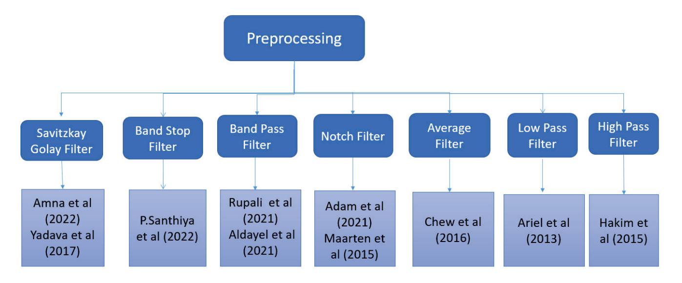
**Figure 1.** Preprocessing of EEG signals in literature.
#### 2.2. Feature Extraction of EEG Signals
Data that has been preprocessed typically consists of large quantities and has higher dimensions. Data presented in this way does not convey any information that is valuable and also provides redundant information. The term "feature set" refers to a subset of data that contains fewer dimensions, and additional processing is done on this feature set. The transformation of data into a feature set is known as feature extraction. When the EEG signals have been preprocessed, features are extracted for the classification between like and dislike states. EEG signals are decomposed by the Daubechies 4 wavelet decomposition in [5]. Abeer et al. [2] extracted features by using PCA. Aldayel et al. [5] splits the coefficients into five frequency bands. Reference [20] used Morlet wavelet transform by using Gaussian 106
*Sensors* **2022**, *22*, 9744
wave shapes. Reference [20] have employed the FFT for feature extractions, and STFT was used by Rakshit et al. [16].
DFT was employed by [23] for feature extraction.The statistical mean was calculated by [21] for all electrode channels, whereas [18] only utilised it for the specific channels. In [21], the Welch method was used for feature extraction. According to Guo et al. [22], there are two ways to estimate rating. One of them is to take the average of the relative power measures among participants, and the other is to simply use the average relative power across participants. The power spectrum density has been extracted by numerous researchers like [19,23–25], and power spectral analysis has been used to obtain spectral moments. In [26], features were extracted by statistical analysis by employing the spectral centroid. Figure 2 shows us the techniques employed for extracting features from EEG signals.
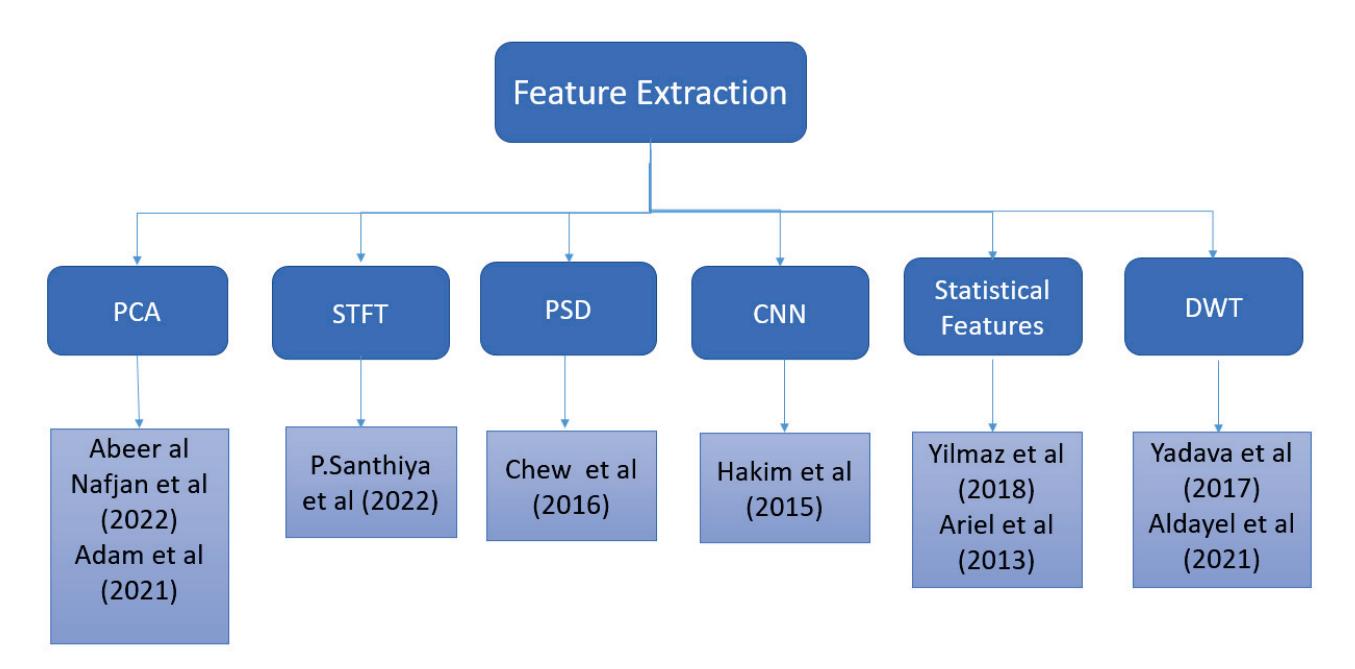
**Figure 2.** Feature extraction of EEG signals in the literature.
#### 2.3. Classification of EEG Signals
Following the completion of the process of feature extraction from EEG signals, the next step is to categorize the signals into the like and dislike states. One definition of classification is the process of developing a model that partitions the data into a number of distinct categories. The values of particular distinguishing characteristics are used to classify the data; samples that belong to the same class as other samples in terms of these characteristics' values are classed together. By using a boosted tree classifier, Amna et al. [27] were able to reach an accuracy of 88.89% when classifying EEG signals. Abeer et al. [2] employed DNN for the classification of EEG signals.
Researchers [25,28] employed RNN for the EEG data classification model. Ref. [29] classified EEG with 92.40% accuracy into four categories of movements (foot, right/left hand, and rest) by using advanced visualization techniques and a convolutional neural network (CNN) [30,31]. In [32] researchers employed a CNN model for classification of EEG signals. Hasnain et al. [33] extracted features from EEG data by using a convolutional deep belief network. The parietal lobe is responsible for touch, taste, and bodily awareness. The prefrontal and frontal lobes have the most influence on neuromarketing [34]. Certain studies focused their efforts on certain brain regions [35], whereas others considered the entire brain [34,36–40].
Ambler et al. [34] discovered that advertisements had an effect on brain activity in diverse cortical areas. Researchers demonstrated the effect of visual stimuli on the activation of the left frontal lobe by using EEG in the study cited in the previous sentence [37]. Dmochowski et al. [41] analyzed EEG data from participants in commercial videos in order to identify regions of the brain that are consistently more (or less) active in response to stimuli. Braeutigam et al. [42] goes into additional depth on both predictable and unpredictable decisions, where predictability is determined by prior use of the product
107
*Sensors* **2022**, *22*, 9744
and the time gap between stimulation and decision making. The multiple brain regions that are related to pleasure and reward were investigated in [43], and the study provides a comprehensive explanation of these brain regions. Researchers used a mix of convolutional neural networks (CNNs) and long short-term memory (LSTM) in [44] to classify emotions based on EEG readings. Figure 3 provides a representation of the classification methods that researchers used in order to divide EEG data into preference categories of like and dislike.
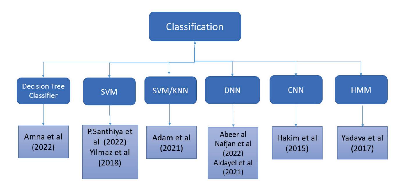
**Figure 3.** Classification of EEG signals in the literature.
Most of the research in neuromarketing and EEG is focused on how consumers feel about products, but here the emphasis is on the details of the product that cause the subject to make a particular choice (see Fernandez et al. [45]). Duan et al. [46] employed PNN and KNN for classification of EEG signals. Brain activation and oscillatory activity between the left and right occipital electrodes were studied by Kawaski et al. [47] to better understand the impact of color preference on the visual attention-related region of the brain. Rakshit et al. [16] employed logistic regression to discover the most distinct frequencies for consumer product choice. Frontal spectral activations of the brain have been explored by looking at the subjects' preferences, as they record them (see Kawasaki et al. [48]). On a diabetic retinopathy dataset, a model composed of machine learning (ML) algorithms such as random forest (RF) classifier, decision tree classifier, adaboost classifier, K-nearest neighbor classifier, and logistic regression classifier is tested by Reddy et al. [49]. Aldayel et al. [5] features are classified into like and dislike by using SVM and RF and obtained an accuracy of 68.33%. Morin et al. [50] conducted research and used the Welch method for classification of EEG signals. Yadava et al. [1] used the HMM for classification of EEG signals in terms of likes and dislikes. Aldayel et al. [5] used the DNN for the classification of EEG signals. In [51], researchers used SVM for the purpose of classification. Luis et al. [52] also used SVM for classification. In Hammou et al. [7], the researchers used RF for classification.
Classification is the ultimate and also the most cardinal step in consumer choice recognition systems [53], as it is the classifier performance that is used to calculate the sensitivity and specificity. Artificial neural networks, deep neural networks, linear discriminant analysis, K-nearest neighbors, RF, and decision trees were mostly used by researchers in existing methods. A comparison of the most recent state-of-the-art consumer choice recognition approach demonstrates that preprocessing of EEG signals is essential for the classification of EEG signals with high sensitivity and specificity. In the feature-extraction process, both handcrafted and automated features can be extracted; nevertheless, it has been noted that automated features outperform handcrafted features.
A combination of both of these characteristics can be advantageous, but it is not currently utilized by researchers in their techniques employed in existing choice recognition systems. Feature selection also minimizes the influence of the curse of dimensionality, which is lacking in current approaches. Furthermore, there is a tradeoff between sensitivity and specificity. Multivariate features can be retrieved, and classification can be
108
*Sensors* **2022**, *22*, 9744
performed by using DNN, SVM, and RF as these classifiers provide improved performance if preprocessing and extraction of features have been performed effectively.
Analysis of the existing state-of-the-art methods has shown that choice recognition cannot be predicted with higher sensitivity without efficient preprocessing, a complete set of features, and effective classification. Existing approaches in all three processes are hindered by numerous research gaps. In preprocessing, many researchers do not use a set of methods to boost the SNR of EEG signals. No technique for EEG signals has offered a solution to reduce the impact of the class imbalance problem on consumer choice recognition. Existing approaches lack a comprehensive feature set, which must be created by combining both handcrafted and automated features, and classification has also been kept simple. Table 1 shows the recent state-of-the-art methodologies for consumer emotion prediction by using EEG signals.
**Table 1.** Comparison of different state-of-the-art customer choice recognition systems.
| Method | Preprocessing | Features | Classifier | Accuracy | Sensitivity | Specificity |
|------------------------------------|------------------------|----------------------|-------------------------|----------|-------------|-------------|
| Amna et al. [13] (2022) | Savitzkay Golay Filter | - | Boosted Tree Classifier | 88.89% | 84.68% | 86.76% |
| Abeer al Nafjan et al. [54] (2022) | bandpass Filter | PCA | DNN | 94% | - | - |
| P.Santhiya et al. [55] (2022) | ICA | NW-STFT | SVM | 91% | 90.23% | 89.97% |
| Somayeh et al. [56] (2022) | ICA | PSD | Statistical Analysis | 93% | - | - |
| Rupali et al. [57] (2021) | bandpass Filter | DWT | LSTM | 92% | 90.36% | 91.86% |
| Adam et al. [14] (2021) | Notch Filter | PCA | SVM, KNN | 68.50% | - | - |
| Aldayel et. al. [4] (2021) | Bandpass Filter | DWT | DNN | 87% | 91.2% | 87.5% |
| Yilmaz et al. [58] (2018) | bandpass Filter | Statistical Features | SVM | 82.55% | 78.63% | 80.79% |
| Jafar et al. [20] (2018) | - | Statistical Features | DT | 68.33% | 67.98% | 66.37% |
| Yadava et al. [1] (2017) | Savitzky- Golay Filter | DWT | HMM | 70% | - | - |
| Teo et al. [17] (2017) | - | DNN | DNN | 74.60% | 71.49% | 73.60% |
| Chew et al. [15] (2016) | Average Filter | PSD | SVM | 80% | 82.3% | 80.5% |
| Maarten et al. [59] (2015) | Notch Filter, ICA | FFT | SVM | 68% | - | - |
| Hakim et al. [52] (2015) | High Pass Filter | Statistical Features | ANN | 68.50% | - | - |
| Ariel et al. [8] (2013) | Low Pass Filter | Statistical Features | Cardinal Analysis | 65% | 61.73% | 64.19% |
#### 3. Materials and Methods
*Dataset Explanation*
The dataset was recorded by [1] by using an Emotiv EPOC+ device and consists of EEG recordings from 25 subjects for 42 different products. Table 2 shows a summary of the dataset. Electrodes placed on the scalp provide different channels of brain signals. A total of 14 electrodes were used for the acquisition of the EEG signals. A sampling frequency of 2048 Hz is used internally in an EPOC and then the data is downsampled to 128 Hz in order to reduce data and speed up computation. Table 2 depicts the details about the neuromarketing dataset gathered by Yadava et al. [1].
**Table 2.** Summary of neuromarketing dataset.
| Number of Participants | 25 |
|---------------------------|----------------------------------------|
| Participants Gender/Age | Both male and females aged 18–38 years |
| No. of Products | 14 |
| No of Samples | 42 $(14 imes 3)$ |
| Total Samples | 42 $ imes$ 25 = 1050 |
| EEG Signal Recording Time | 4 s |
109
*Sensors* **2022**, *22*, 9744
**Table 2.** *Cont.*
| EEG Signal Recording Time | 4 s |
|---------------------------|-------------------------------------------------------------------------------------------------------------------------------|
| No of Classes | 2 (Like & Dislike) |
| No of Channels | 14 |
| EPOC Sampling Frequency | 2048 Hz to 128 Hz |
| Device Name | EMOTIV EPOC |
| Device Name | EMOTIV EPOC |
| Experimental Method | Each user viewed and evaluated his or her pref
erences for 42 pictures of ecommerce products
in form of like or dislike |
#### 4. Overview of Proposed Methodology
In the proposed method, preprocessing involves artifact removal and noise removal using the Savitzky–Golay filter. This filter is solely responsible for smoothing EEG signals. Smoothing data is a method of removing noise from a set of data. It enables the creation of a pattern that stands out from the ambient noise. A band stop filter has been applied on this frequency domain data to remove noise. The SMOTE algorithm is also employed to deal with the class imbalance problem.
SMOTE makes use of the vector interpolation approach in order to produce synthetic samples of the minority class when working with high-dimensional data. Following the completion of the preprocessing, the features are extracted through the use of the power spectral density (PSD), also known as the Welch method, and the discrete wavelet transform as examples of handcrafted features, and long short-term memory (LSTM)-based features as examples of automated features. In signal processing applications, LSTM is extensively applied to extracted automated features. After extracting features from denoised EEG signals, the training data was 70% and testing data was 30%. Different ML classifiers were employed, including decision tree (DT), SVM, and deep learning classifiers (DNNs) for classification between the two classes. However, it is observed that the ensemble classifier gives better classification results in terms of increased sensitivity and specificity. Figure 4 shows us the proposed ensemble model for consumer emotion prediction by using EEG signals.
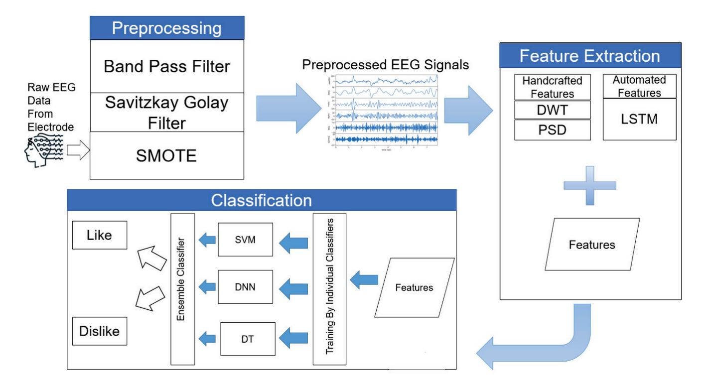
**Figure 4.** Flow diagram of the proposed consumer emotion prediction.
110
*Sensors* **2022**, *22*, 9744
*Proposed Preprocessing of EEG Signals*
EEG recordings are easily influenced by external noise. It is difficult to pinpoint the features in EEG signals due to noise. There are a variety of known solutions to the noise problem. Smoothing data is a method of removing noise from the EEG signals to increase the signal-to-noise ratio. It enables the creation of a pattern that stands out from the ambient noise. Noise was removed from EEG signals by using the Savitzky–Golay filter that smoothes the signal and removes the noise. FFT and the Savitzky–Golay filter were employed to reduce noise and remove artefacts. A Savitzky–Golay filter is a digital filter that can be used to a range of digital data points to smooth them out to increase their precision without affecting the signal. In the dataset, there are two classes, like and dislike. Another problem is the like-to-dislike samples ratio, which indicates that there are very few samples of the like class available in the dataset in comparison to the samples available for the dislike class. This leads to a class imbalance problem, which in turn hinders the classification's performance.
As part of the proposed method, synthetic data for the like class has been generated in order to lessen the impact of the class imbalance between the like and dislike classes. To overcome the problem of class imbalance, SMOTE was employed to generate the samples for the like class. In the SMOTE technique, the oversampling technique was employed, in which the data of the minority class was duplicated from the majority class population. SMOTE works by using a *k*-nearest neighbor algorithm to make synthetic data samples for the minority class. The samples are exactly the same as the original samples. SMOTE works on selecting instances in the feature space that are close to each other, drawing a line between them, and then drawing a new sample along that line. First, an example from the minority group is selected randomly. Then, *k* of the nearest neighbors for that case (usually *k* = 5) are discovered. Synthetic samples are constructed at random points between the two samples in feature space, based on a random selection of a neighbour.
After applying the SMOTE technique and removal of noise to increase the SNR, the frequency was resampled to a 128 Hz channel. In contrast to previous findings, preference states seem to generate low-frequency EEG signal ranges primarily. Thus, the useful bandwidth of the EEG signal data for choice detection is between 4 and 45 Hz. A bandpass filter with a bandpass of 4.0 to 45.0 Hz was applied. Savitzky–Golay filters accept a variety of input parameters, including *X*, order, and frame length. We employed a Savitzky–Golay filter with an order of 11 and a frame length of value 2. To eliminate noise from all 1050 files, a Savitzky–Golay filter was employed. We have
Qj = \sum\_{i=-\frac{m-1}{2}}^{\frac{m-1}{2}} c\_{i} S\_{j+1}, \quad \frac{m+1}{2} \le j \le n - \frac{m-1}{2}
(3.1)
$$\tag{1}$$
where *m* is the number of frames, *ci* is the number of convolution coefficients, and *Q* is the smoothed signal. Polynomial values are calculated with the frame span *m*, which is used to find the values of *ci* with this method.
#### 5. Proposed Feature Extraction of EEG Signals
Feature extraction is the process of getting lower-dimension, useful, and nonredundant information from the data. This reduced set of information is known as the feature vector. Automated feature extraction techniques and handcrafted feature-extraction methods were employed for getting better results. Feature extraction is a procedure that enhances the complexity of raw EEG signals, and by the help of feature extraction, one easily gather required information from the EEG signal. Many time-frequency domain feature-extraction approaches are available. Wavelet transform (WT) for EEG signals is now the most common and useful option. The proposed method calculates features in both domains like the time domain and frequency domain.
111
*Sensors* **2022**, *22*, 9744
#### 5.1. Handcrafted Features
The preprocessing of EEG signals is followed by feature extraction. Discrete wavelet transform and power spectral density are handcrafted features extracted from EEG signals. DWT encodes the signal in the time-frequency domain and are usually applied in biomedical signal processing. When it comes to decomposition, the DWT method uses a multistage approach to break down an input signal into smaller waves.
Wavelet transform methods are of two types, namely CWT and DWT [60]. DWT stands for discrete wavelet transform, and it is a wavelet transform that samples wavelets by using scaling and translation parameters. The wavelet vector decomposes the signals into orthogonal components (see Nilashi et al. [60]). The DWT technique derives a collection of features, which includes details (D2-D5) and (A5). The signals are decomposed into wavelet coefficient vectors, which are then analyzed. Both time and frequency domains are considered in this technique. The following two equations describe the sequential filtering of the initial signal, which begins with low-pass filtering *g* and ends with high-pass filtering *h*. The wavelet function can be seen as in following equations,
$$\int_{+\infty}^{-\infty} \psi(t)dt = 0 \quad (2)$$
$$\varphi_{m,n}(t) = a_0^{-\frac{m}{2}} \varphi(a_0^{-m} t - nb_0), \tag{3}$$
where *a* and *b* are scaling and translation parameters that can have discrete values. *m* is frequency and *n* is time belonging to *Z*. *A* and *D* are shown in the scaling function (4), and (5) denotes the wavelet function. We have
$$\phi_{j,k}(n) = 2^{j/2}h(2^{j}n - k) \tag{4}$$
w\_{j,k}(n) = 2^{j/2}g(2^{j}n - k).
$$(5)$$
(*φk*), *k*(*n*) denotes the scaling function that belongs to (L), and (*ωj*), *k*(*n*) denotes the wavelet function that is related to (*H*); the signal's length is denoted by *M* Here, *n* is the discrete variable that lies between the values of 0 and *M-1* and here we have *J* = (log 2) (*M*) and the values of *k* and *j* are between *0-J-1*. Equations (6) and (7) are used to calculate the values of *Ai* and *Di* [27],
$$A_i = \frac{1}{\sqrt{M}} \sum_{n} x(n) \times \phi_{j,k}(n) \quad (6)$$
$$D_i = \frac{1}{\sqrt{M}} \sum_n x(n) \times \omega_{j,k}(n). \tag{7}$$
Figure 5 shows the four-level decomposition of EEG signals. A second featureextraction method utilised is PSD. Fourier analysis demonstrates that every physical signal may be reconstructed into a spectrum of frequencies spread across a continuous range. The signal's frequency content, including noise, is called its spectrum. When a signal's energy is focused in a certain time span, the energy spectral density can be computed. The PSD can be defined as the energy distribution per unit time in a signal because the total energy of a signal throughout all time is limitless.
The PSD indicates the strength of a signal by its frequency. PSD is a technique that is widely used in neuromarketing research is feature extraction by frequency domain analysis [61]. For determining power spectral density of EEG signals, MATLAB was used.
112
*Sensors* **2022**, *22*, 9744
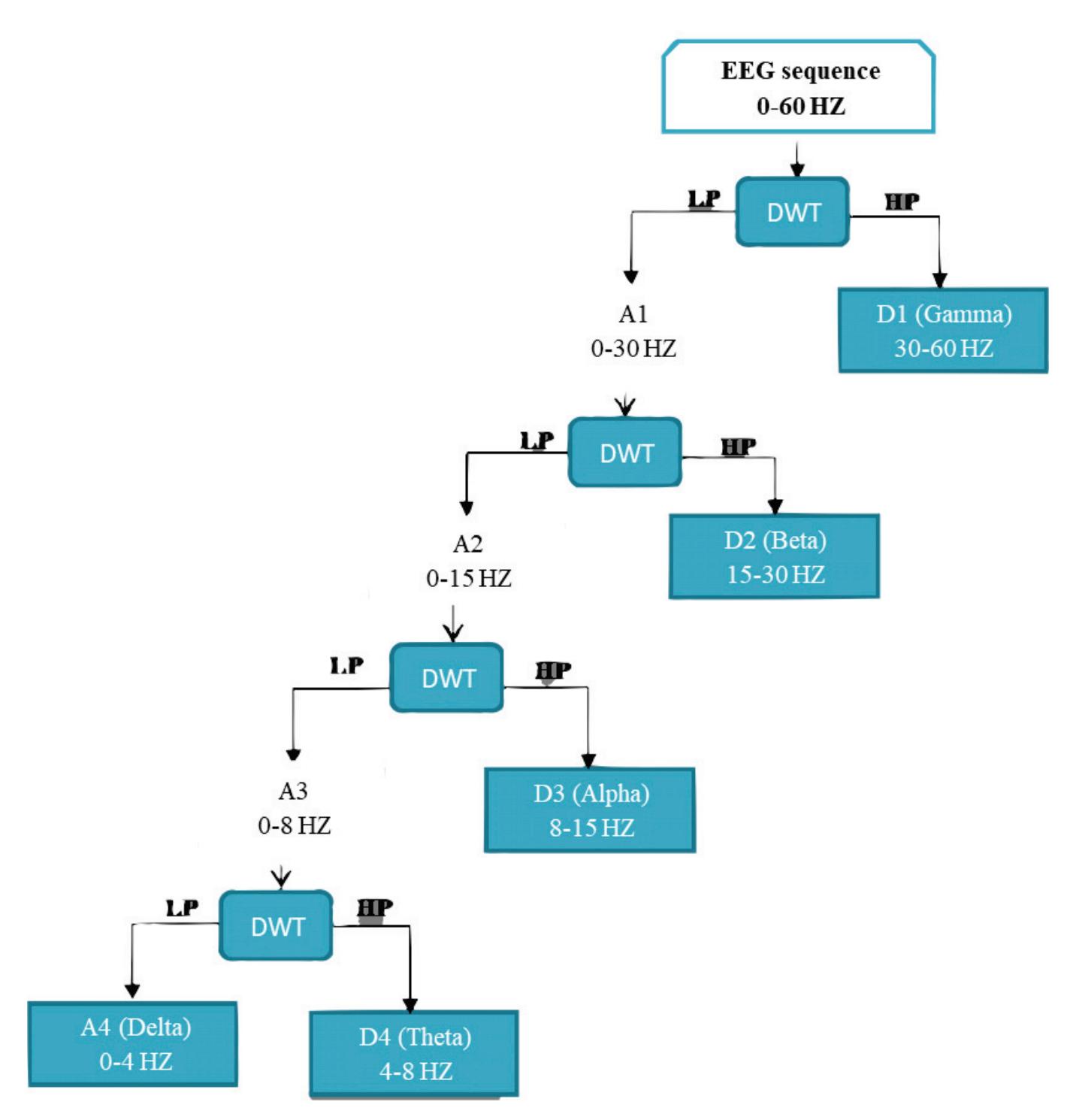
**Figure 5.** Decomposition of EEG signal into four levels by using DWT.
#### 5.2. Automated Feature Extraction by Using LSTM
Predictive problems using time series data are notoriously challenging to implement due to their inherent complexity. Time series predictive modeling adds more complexity than traditional regression predictive modeling because it includes a sequence dependence among the input variables. One of the most effective types of neural networks, recurrent neural networks, are able to take sequence dependency into account. Recurrent neural networks like the LSTM network are popular in deep learning because they allow for the successful training of extremely massive architectures. The inability to selectively remember essential information or values for a longer period of time causes feed-forward neural networks and non-LSTM recurrent neural networks to be less effective at sequence prediction.
In 1997, Sepp Hochreiter and Jürgen Schmidhuber published the recurrent neural network (RNN) architecture known as LSTM [62]. When it comes to learning from experience, conducting analysis, and making predictions about time series data, LSTM networks excel in comparison to traditional RNNs. Several iterative enhancements have been made to LSTM designs over the years. The LSTM architecture relies heavily on the idea of gated cells. The architecture of the cell allows LSTM to handle long-term dependence by regulating the influx and egress of data. There is a cell state and three gates in an LSTM cell. Figure 6 shows the architecture of the LSTM model employed for automated feature extraction.The
113
*Sensors* **2022**, *22*, 9744
purpose of the sigmoid function used by each gate is to either add or subtract data from the current state of the cell.
**Figure 6.** Architecture of LSTM model [36].
A memory cell is composed of four primary elements: an input gate, a neuron with a self-recurrent connection, a forget gate, and an output gate. These elements work together to form the cell. A memory cell's state is guaranteed to be stable from one time step to the next thanks to the self-recurrent link's weight of 1. The gates control how the memory cell communicates with its surroundings. The state of the memory cell can be altered by external signals, which can be allowed or blocked by the input gate. In contrast, the state of the memory cell can either impact other neurons or be blocked by the output gate. Both of these outcomes are possible. The forget gate has the ability to alter the self-recurrent link that is present in the memory cell, causing the cell to either remember or forget its former state.
#### 5.3. Significance of Using LSTM for Automated Features
In recent years, deep learning and machine learning technologies have gained prominence, with considerable impacts seen in real-world applications such as image/speech recognition, NLP, classification, prediction, and a wide variety of other applications [63]. The development of artificial neural networks has made these kinds of things conceivable in recent years. RNNs, which are one sort of advanced artificial network, have a great deal of flexibility as a result of their capacity to carry out operations on sequences. When it comes to understanding data patterns that change over the course of time, an RNN is the best option. It is widely acknowledged in the field of data science that the prediction and categorization of sequences is one of the most difficult problems to solve. In time series data, these challenges can range from estimating sales to seeing trends in stock
114
*Sensors* **2022**, *22*, 9744
market data, from comprehending movie plots to recognizing voice tones, from translating languages to predicting a typist's next word on the keypad of an iPhone, etc. In light of current developments in data science, it has come to light that LSTM networks are the most efficient solution to the vast majority of these sequence prediction or classification issues.
The fully connected layer in an LSTM is used to extract robust and relevant features, whereas the Softmax layer in LSTM is used to extract predicted labels in output. Due to the RNN's recurrent structures, LSTM has a low computational complexity when using gradient-based learning techniques to train a neural network. Vanishing gradient is a typical problem that hinders the network's capacity to learn and perform. Although RNNs provide a great deal of resilience, their limited memory means they are vulnerable to vanishing gradients. In order to fix this, a more suitable structure, such as an LSTM is required. The latter is a complex design that overcomes vanishing gradient problems; it is a version of an RNN. Remembering the previous inputs is essential because the output is based on those inputs. When more parameters are introduced, the standard RNN's inability to look back more than a few time steps hinders its performance. An LSTM may selectively forget and remember data/patterns for very long period of time. The ability of an LSTM to detect and prioritize which input and information should be kept within the network sets it apart from more basic RNNs and feedforward neural networks.
#### 6. Proposed Classification
After the successful completion of the training process of automated features by LSTM and handcrafted features by using DWT and PSD, the data was passed to our hybrid classifier. The hybrid classifier combines the weights of SVM, DT, and the deep learning classifier DNN. It gives the findings of each individual classifier a weight and then utilizes this weight-probabilistic ensemble for further processing. The data that was utilized for training is 70% and testing was done on 30% of the data comprising two labels, namely like and dislike. Figure 4 depicts the proposed ensemble framework for the hybrid classifier. The proposed methodology consists of classifiers, namely SVM, DT, and DNN. A genetic algorithm is used to optimise the weights in this weight vector. The weight-modelling process is divided into two stages. The separation of incorrect samples from the rest of the samples in the training dataset is done in the first phase. When individual classifiers classify samples, they classify them into distinct classes, resulting in incorrect samples. These samples were employed alone for optimisation purposes. As we know that processing only the confused samples requires less time, the weights for the confused samples determined in the previous step are optimised in the second phase and optimization of weights was done by genetic algorithm. The detailed working of individual classifiers are as follows.
Decision tree refers to a method of supervised learning that is nonparametric and can be used for both classification and regression. The characteristic that results in the greatest increase of information is chosen to serve as the root node for the [64] structure. Information gain is defined as the anticipated decrease in entropy that is brought about as a result of dividing the samples up according to this characteristic. The following equation can be used to determine the entropy of a system. We have
$$Entropy = -\sum P_i \log_2(P_i), \tag{8}$$
where *Pi* is the ratio of elements in of each label in a set.
The SVM refers to a group of supervised learning algorithms that can be used for classification, regression, and the identification of outliers. SVM is useful in high-dimensional spaces, and their usefulness does not diminish even in circumstances in which the number of dimensions exceeds the number of samples. However, the fundamental concepts that underpin the SVM algorithm can be described in a way that does not involve the use of equations. We have
115
*Sensors* **2022**, *22*, 9744
$$k(x,y) = \exp(-||x - y||^2 / \sigma^2)$$
(9)
$$k(x,y) = (ax \\cdot y + b)^n$$
(10)
$$f(x,y) = \exp(-a|x - y| + b)$$
(11)
$$k(x,y) = (a||x-y||+b)^{1/2} \\ (12)$$
$$k(x,y) = (a||x-y||+b)^{-1/2}
(13)$$
These equations are for the different kernels for SVM. In the SVM, separating hyperplanes are selected based on their margins, which are defined as the distances from the separating hyperplane to the nearest expression vector. By using this hyperplane, the SVM is better and can be able to anticipate the right categorization of samples that have not been seen before.
Once the removal of noise from the data is complete, we split the data by using the train–test split into 70% for training and 30% of the data for testing purposes. We do this before feeding this data to the deep learning model for extraction of features. The number of epochs, also called hyperparameters, is 300. Before starting the training process, the values of hyperparameters must be defined, these values express the model's layer size and decides how the model is being trained.
The hyperparameters that are defined for the DNN classifier are batch size = 100 and epochs = 300. These defined hyperparameter values are optimal, but in some cases these values may not be optimal. Hence, along with the tuning of these sets of hyperparameter values, we have obtained optimal results; this procedure is called hyperparameter tuning. The loss was found with an optimizer which reduces the loss function. Adam is an optimization algorithm for stochastic optimization. For binary class classification, the binary class entropy was employed. An algorithm called binary cross-entropy evaluates each prediction to the actual class output, which can be either 0 or 1. It then creates a score that penalizes the probability based on the difference between the expected and actual values. Increasing cross-entropy loss occurs when the anticipated probability diverges from the actual label. A comprehensive feature vector can be obtained by first extracting the automated features from EEG signals. DNNs are models that are made up of layers of "neurons" that are connected together and in which each layer performs a linear change to the input data. A nonlinear cost function is used to handle the transformation results of each layer after they have been transformed in each layer. By minimizing a cost function that describes the transformation, one can establish how the parameters of such transformations should be set. The applications of deep learning covered an extremely broad spectrum, including areas like as speech recognition, image recognition, and the processing of natural languages. It has been demonstrated that DL is an excellent method for analyzing EEG signals. To detect the consumer preference in terms of likes and dislikes, a model is built based on handcrafted and automated features extracted by DWT, PSD, and LSTM.
The DNN model is a feed-forward neural network with five hidden layers which are fully connected. The input layer has 512 input units, whereas each subsequent hidden layer had 20% of the previous layer units. The activation that was employed is a rectified linear unit (ReLu). The cross-entropy function or cross-functions was employed to calculate the output was SoftMax. The number of target preferences (2) was correlated to the dimension(s) of the output layer. As we are detecting two states from EEG signals, like and dislike, we have two units in our output layer. We have employed the Adam gradient descent on the DNN classifier to train it with the following characteristics: three different objective loss functions (binary cross-entropy, categorical cross-entropy, and hinge crossentropy). The dropout rate for the input layer and hidden layer was 0.3%. We have also used the early stopping criteria to overcome the overfitting. The test set had around 30% of the samples in the dataset; therefore we tested our classifier on it.
116
*Sensors* **2022**, *22*, 9744
*Ensemble Classification by Using the Genetic Algorithm*
After the successful feature extraction, two types to features were gathered. The first one is handcrafted features extracted by DWT and PSD, and the second are automated features using LSTM. The proposed methodology consists of classifiers, namely SVM, DT, and DNN. Weight optimization was carried out by using the genetic algorithm. It gives the findings of each individual classifier a weight and then utilizes this weight-probabilistic ensemble for further processing. As illustrated in the equation below, the classification is dependent on the measurement of evidence supplied by the individual classifiers. We have
$$class(v) = \underset{class_i}{\operatorname{argmax}} \left( \sum_{i=0}^{c} a_k \cdot P(c_k(y = class_i|v)) \right) \quad (14)$$
where *Pck*(*y* = *classi*|*v*) is basically the probability of class i, which gives us the sample node by using the classifier denoted by *k* and the weight is denoted by *ak* that is linked with the probabilistic prediction of the sample belonging to class *Ck*. The data that was utilized for training is 70% and testing was done at 30% of the data comprised of two labels, namely *X*1 = *Like* and *X*2 = *Dislike*. Figure 7 depicts the proposed ensemble framework for hybrid classifiers. The framework includes an ensemble of feature vectors: *ak* = *aDNN*, *aSVM*, *aDT*. Optimization of the weights in this weight vector was done by using the genetic algorithm. Two steps are involved in the modeling of weights. In the first phase, confused samples are separated from the rest of the samples contained in the training dataset. Confused samples are those samples that are categorized to distinct classes by their respective classifiers. As it is easy and requires less time to process only the confused samples, in the second phase, the weights for the confused samples that were computed in the first phase are optimized. The optimization of weights is carried out by using the genetic algorithm.
Figure 7 shows us the block diagram of ensemble classifier. The genetic algorithm is one of the methods that can be used to eliminate redundant or irrelevant features. In machine learning, often redundant or irrelevant features obscure the primary categorization features. Feature selection has become an important area of study in order to eliminate such characteristics that are unnecessary. The feature-selection process is to select some of the most effective and representative features from a set of features in order to achieve the purpose of reducing the feature space dimension. The genetic algorithm is useful for selecting features. The selection is based on the new individuals' physical fitness. The genetic algorithm is founded on the idea that the greater the fitness, the greater the probability of selection. With low fitness, the probability of selection is low. This selection technique produces a relatively optimum group from the initial data. The selected individuals then undergo the crossover procedure to produce new individuals. The subsequent step is mutation, which yields a new subset. Through this series of processes, a new generation of individuals is produced that is unique from the original generation and is progressing toward an increase in overall fitness from one generation to the next. As a result of the decision to generate the future generation by picking the individuals that are fit, the less fit individuals would be gradually removed. We have
$$P(x_k^i) = \frac{f(x_k^i)}{\sum_{i=1}^{n} f(x)_k} \cdot$$
(15)
Figure 7 shows the weights optimization of classifiers like SVM, DNN and DT.
117
*Sensors* **2022**, *22*, 9744
**Figure 7.** Block diagram of ensemble classifier.
#### 7. Performance Evaluation
To verify the validity of the proposed system, different performance evaluation criteria have been used. These included sensitivity (the true positive rate), specificity (the true negative rate), and ROC (the receiver operating characteristic curve). Accuracy is the measure of correctly classified samples. Accuracy cannot be a good measure of evaluation in our case because even if the system does not correctly identify the positive (which is less in number) but correctly identifies all the instances of the negative class (which has a higher proportion), the accuracy will still be high. Another reason is that with the increase in sensitivity, the false positive rate also starts to increase, measurement of metrics like sensitivity and specificity are required of evaluate our system for classification of samples between the like and dislike states.
• **Accuracy** Classification models can be evaluated by using a variety of criteria, and one of them is accuracy. Accuracy is the percentage of correct predictions out of all possible predictions. The proposed model considers accuracy to be a measure of the model's ability to accurately predict whether the consumer will like the product or dislike the product. The accuracy can be calculated by using Equation (22):
Accuracy =
$$\frac{TN + TP}{TN + TP + FN + FP}$$
(16)
In the above equation, *TP* means the true positive and *FN* indicates the false negative. • **Sensitivity** The percentage of correct positive predictions is what we call sensitivity.
Higher sensitivity in a proposed model denotes the model's ability to accurately predict whether or not the customer will like the product. Equation (23) can be used to calculate sensitivity:
Sensitivity = $\frac{TP}{TP + FN}$
(17)
• **Specificity** The degree of specificity refers to the validity of negative predictions, or the percentage of true predictions. With a better model, we can forecast that a consumer will not like a product with greater accuracy. Equation (24) can be used to calculate sensitivity. We have
$$Specificity = \frac{TN}{TN + FP'}$$
\tag{18}
where *TN* means the true negative and *FP* indicates the false positive. To conclude, the average specificity of the ensemble classifier is better than the average specificity of DT, SVM, and DNN.
118
*Sensors* **2022**, *22*, 9744
#### 8. Results and Discussion
In this section, we present the results of our investigation as well as an explanation of the methodology that we have proposed. After the preprocessing and feature extraction, the weights of classifiers like DT, SVM, and DNN were optimized by using the genetic algorithm. Results were compared in terms of the area under curve, accuracy, sensitivity, and specificity, the proposed method is compared with other classifiers, including DT, SVM, and DNN.
An SVM is a type of supervised machine learning model that uses classification techniques in order to categorize samples into one of two groups. After providing an SVM model with training data for each category, it is possible to train the model to categorise fresh data by using the training data. They offer two significant advantages over more recent algorithms such as neural networks: increased efficiency with a lower sample size and faster speed than the older techniques (in the thousands). Because of this, the approach is suitable for text classification tasks, which need a dataset consisting of at least several thousand cases that have been labelled. In the field of machine learning, the measuring of performance is a very important component. The AUC-ROC curve is a useful tool for assessing the performance of classification algorithms. An area under the receiver operating characteristic curve (AUC-ROC) is used to visualise the performance of binary class classifiers.
Of the several approaches to evaluation, the ROC curve is by far the most useful. Sometimes it is also referred to as the area under the receiver operating characteristic (AUROC). The AUC-ROC curve is a useful tool for evaluating the performance of a classification task at a number of different thresholds. When it comes to the ability to separate measurements, the area under the curve (AUC) is the symbol for it, whereas the probability is generated from the ROC curve. When the area under the curve (AUC) is greater than 0.8, it indicates that the model does an excellent job of predicting the proper answer. When plotting the ROC curve, the x-axis indicates the rate of false positives, whereas the y-axis indicates the rate of true positives. As long as the AUC is close to 1, a model is likely to stand out, and when the value of the AUC approaches 1, a model is functioning in a very good way for binary class classification. If the AUC is getting close to 0, it suggests that the model's output is not very accurate, and is not satisfactory. It suggests that our model is incorrectly forecasting the values 0 and 1, respectively.
Figure 8 depicts the AUC curve of the classifier. In the proposed methodology, we have compared the accuracy with different classifiers which include decision tree, SVM, DNN, and the proposed hybrid classifier. Among the different classifiers, the hybrid classifier outperforms in terms of accuracy and gives us highest accuracy of approx 96.68%. The sensitivity is also a very important feature to evaluate the performance of the model.
**Figure 8.** AUC curve to examine the performance of ensemble classifier.
119
*Sensors* **2022**, *22*, 9744
#### 9. Result Achieved by Varying Different Experimental Settings
The proposed deep learning model is employed on the mentioned data with the goal of recognition of customer preference in terms of likes and dislikes. The experiment started by preprocessing the data to reduce the data by removing unnecessary information and also noise present in the data. In contrast to previous findings, preference states seem to generate a low-frequency EEG signal. Thus, the useful bandwidth of EEG signal data for preference detection is between 4 and 45 Hz. We have devised three different experiments.The subsequent sections describe the experiment's goal, the steps that were taken, and the results that were found in each experimental setting.
#### 9.1. Analyzing the Effect of Various Preprocessing Techniques in the Proposed System
Increasing the signal-to-noise ratio (SNR) of EEG signals is a key step in the customer preference recognition technique because it lowers noise and other distortions in the signals. EEG signals have been preprocessed by using a variety of approaches to boost SNR and eliminate power line noise. Bandpass filtering, fast Fourier transform (FFT), Savitzky– Golay filter and synthetic data generation are all examples of these approaches. First, the EEG signals were not preprocessed in order to evaluate the performance of the baseline feature-extraction method. By using time/frequency domain characteristics obtained from the data, states of liking and disliking are categorized by using an SVM classifier. Accuracy, sensitivity, and specificity are used to evaluate the experimental environment. Table 3 shows the analysis and comparison of various preprocessing techniques for removal of noise and checks the performance metrics like accuracy, sensitivity, and specificity.
**Table 3.** Comparison of different preprocessing techniques in terms of accuracy, sensitivity and specificity.
| Method | Accuracy% | Sensitivity% | Specificity% | Precision% | F1 Score% |
|--------------------------------------------|-----------|--------------|--------------|------------|-----------|
| No Preprocessing, DWT, SVM | 63.48 | 62.79 | 62.68 | 63.46 | 63.59 |
| FFT, DWT, SVM | 68.52 | 67.96 | 67.91 | 69.5 | 68.97 |
| FFT + Savitzkay Golay Filter, DWT, SVM | 71 | 70.58 | 70.24 | 71.76 | 70.3 |
| FFT+Savitzkay Golay Filter+SMOTE, DWT, SVM | 76 | 75.46 | 75.71 | 74.98 | 75.3 |
A consumer preference recognition system that does not preprocess EEG signals is unable to obtain improved results. In this experimental setup, we could not achieve a sensitivity and accuracy of more than 70%, with 67.2% sensitivity, and 69.5% specificity. From experiment 1, we concluded that without the preprocessing of EEG signals we could not achieve good results, so in the second experiment a bandstop filter was employed to remove the high frequency components. After applying the bandpass filter and Savitzky– Golay filter and SMOTE technique, an experiment was conducted to check the effect of the preprocessing technique. In the second experiment, it was concluded that by using preprocessing techniques the accuracy improved to 76%.
Figure 9 shows us the comparison of difference preprocessing techniques in terms of specificity, sensitivity, and accuracy.
120
*Sensors* **2022**, *22*, 9744
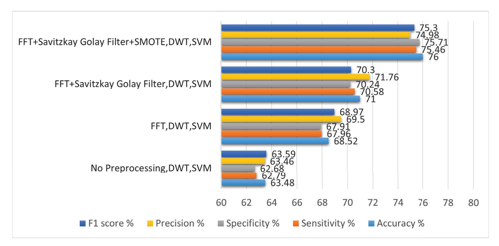
**Figure 9.** Analysis of different preprocessing techniques in the proposed system.
#### 9.2. Examining the Effects of Different Feature-Extraction Methods in the Suggested System
In the second experiment, the optimal method for extracting features from a dataset is examined. The handcrafted features and automated features were tested in this experiment. The handcrafted features include the DWT and power spectral density (PSD), and automated feature include LSTM-based features. Both the handcrafted and automated features were tested one by one, and results were evaluated by accuracy, specificity, and sensitivity. An additional factor is that the automated features were extracted by using LSTM.
In the first iteration, the preprocessing settings were retained the same as they were in the first experiment, and the DWT was utilized in order to extract the features. SVM was employed for classification after feature extraction. This method's outcomes cannot be compared to what is currently possible. The experiment had a 62.79% sensitivity and a 62.68% specificity. PSD was used instead of DWT in the second iteration, and preprocessing settings were identical to the first experiment. After the feature extraction, classification was done by SVM. As a result of this adjustment, the sensitivity was increased to 78.87%, and the specificity was increased to 78.69%. In the third iteration, DWT- and PSD-based features were concatenated, the preprocessing and classification setting was the same as per a previous experiment. In this iteration, the accuracy achieved was 87.25%, the specificity was 87.78%, and the sensitivity was 87.66%.
Table 4 shows us the comparison of different feature-extraction techniques. In order to better understand the implications of various feature-extraction methods, we designed an LSTM network. The results produced in this environment were somewhat comparable to those of current state-of-the-art systems. After a thorough investigation, similar architectures were also discovered in the literature. The details of this network have been explained in detail in chapter 3. The experimental settings produced the increased accuracy of 85% with specificity of 84.78% and sensitivity of 84.27%. In the last iteration, DWT-, PSD-, and LSTM-based features were gathered, passed to the SVM classifier, and the preprocessing settings were the same as per previous iterations. The accuracy achieved in this experiment was 87.25%, the sensitivity was 87.66%, and the specificity was 87.66%.
121
*Sensors* **2022**, *22*, 9744
**Table 4.** Comparison of different feature extraction techniques applied.
| Method | Accuracy% | Sensitivity% | Specificity% | Precision% | F1 Score% |
|----------------------------------------------------------------|-----------|--------------|--------------|------------|-----------|
| FFT + Savitzkay Golay Filter + SMOTE,
PSD, SVM | 79.26 | 78.87 | 78.69 | 79.63 | 79.52 |
| FFT + Savitzkay Golay Filter + SMOTE,
DWT + PSD, SVM | 83.28 | 82.91 | 82.86 | 83.2 | 83.7 |
| FFT + Savitzkay Golay Filter + SMOTE,
LSTM, SVM | 85 | 84.27 | 84.78 | 84.6 | 85.3 |
| FFT + Savitzkay Golay Filter + SMOTE,
DWT + PSD + LSTM, SVM | 87.25 | 87.66 | 87.78 | 88.6 | 87.8 |
Figure 10 shows us the comparison of feature extraction techniques.
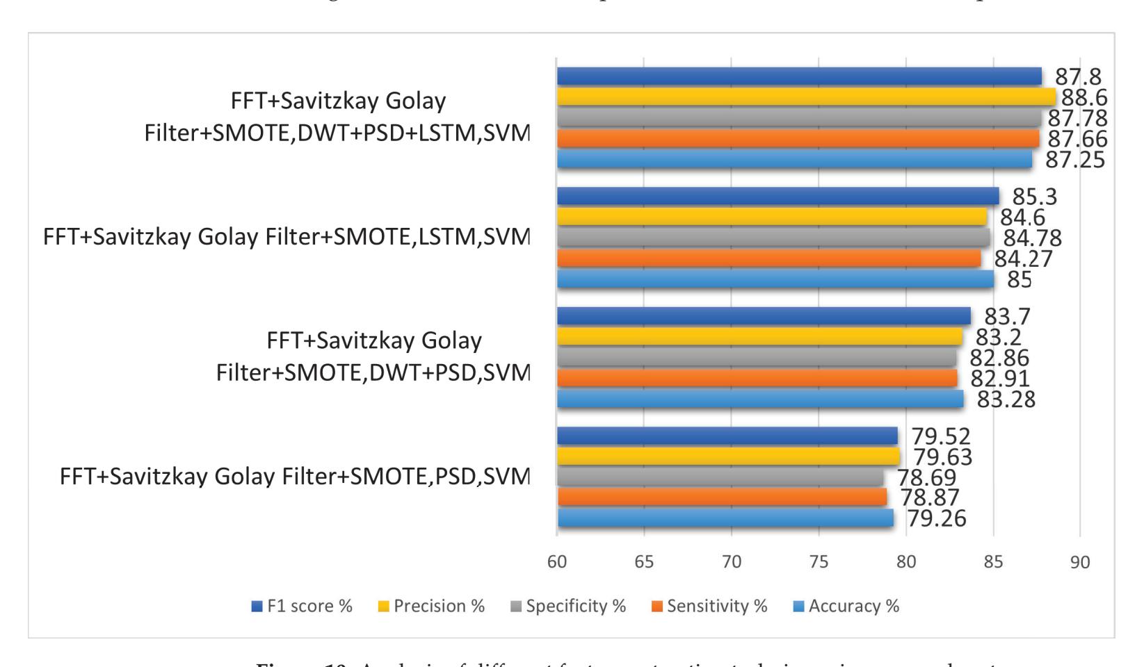
**Figure 10.** Analysis of different feature extraction techniques in proposed system.
*9.3. Analysis of Effect of Various Classification Techniques in the Proposed System*
Different classifiers were tested as part of a third experimental setting. Preprocessing was handled by Savitzky–Golay filter, SMOTE, and FFT. Feature extraction was handled by DWT and PSD, and LSTM.
DNN was employed to classify in the first iteration. Decision tree was utilised for the classification in the second iteration, and SVM was employed in the third iteration and didn't get the accuracy. For this reason, weights for all the classifiers are gathered and passed to the genetic algorithm for optimization and then classification between like and dislike was done by optimized weights. The following are the classification results obtained after optimization: a sensitivity of 95.89%, specificity of 96.21%, accuracy of 96.89%, precision of 95.78%, and F1 score of 95.76%. Table 5 summarises the initial conditions and the subsequent outcomes for each iteration.
122
*Sensors* **2022**, *22*, 9744
**Table 5.** Comparison of different classification techniques in terms of accuracy, sensitivity, specificity, precision, and F1 score.
| Method | Accuracy% | Sensitivity% | Specificity% | Precision% | F1 Score% |
|---------------------------------------------------------------------------------------------------------|-----------|--------------|--------------|------------|-----------|
| FFT + Savitzky-Golay Filter + SMOTE,
DWT + PSD + LSTM | 90.89 | 90.78 | 92.27 | 91.5 | 91.8 |
| FFT + Savitzky Golay Filter + SMOTE,
DNN | 92.47 | 90.43 | 91.37 | 92.5 | 91.89 |
| FFT + Savitzky Golay Filter + SMOTE,
DWT + PSD + LSTM Ensemble
Classifier Using Genetic Algorithm | 96.89 | 95.89 | 96.21 | 95.78 | 95.76 |
Figure 11 shows us the comparison of different classification techniques.
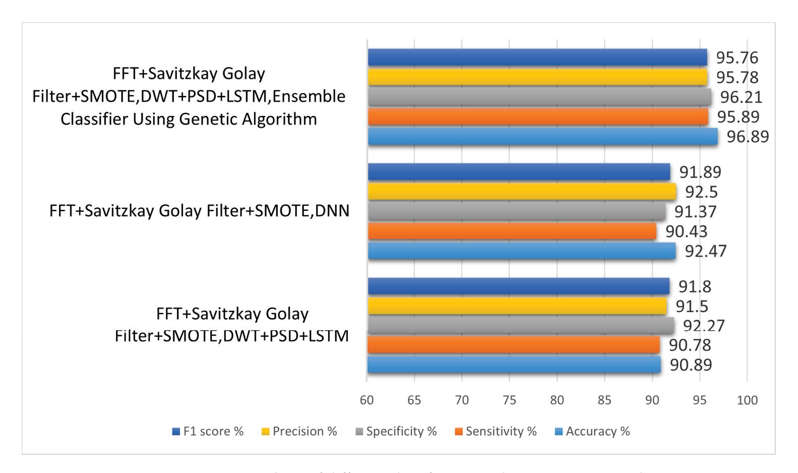
**Figure 11.** Analysis of different classification techniques in proposed system.
#### 10. Comparison of Results of Consumer Choice Recognition Method by Using Different Experiments
Following the first three experiments, the preprocessing of EEG signals was determined. Figures 4–11 compares the results of various experiments conducted as part of this study. In the first experiment, EEG data was used with no preprocessing to extract handcrafted features, which were then classified by using SVM. In the second experiment, EEG signals were preprocessed by first applying bandpass filtering to eliminate high-frequency components; then, handcrafted features were extracted and applied SVM to classify them. The comparison of these two trials reveals that preprocessed signals yield significantly better results with improved accuracy. Following the previous experiment, EEG signals are preprocessed by using a bandpass filter and Savitzky–Golay filter and FFT in the third experiment. In this experiment, the same method was employed for feature extraction and classification as previously used in other experiments. With this experimental setup, there are improvements in accuracy, sensitivity, specificity, precision, and F1 score. Similar to experiment 4, experiment 5, and experiment 6, feature-extraction methods have been modified by adopting the same preprocessing and classification technique. Table 6 depicts the comparison of results for different experimental settings by evaluating in terms of accuracy, sensitivity, specificity, precision, and F1 score.
123
*Sensors* **2022**, *22*, 9744
**Table 6.** Comparison of different experimental settings applied.
| Method | Accuracy% | Sensitivity% | Specificity% | Precision% | F1 Score% |
|-------------------------------------------------------------------------------------|-----------|--------------|--------------|------------|-----------|
| No Preprocessing, DWT, SVM | 63.48 | 62.79 | 62.68 | 63.46 | 63.59 |
| FFT, DWT, SVM | 68.52 | 67.96 | 67.91 | 69.5 | 68.97 |
| FFT + SGF, DWT, SVM | 71 | 70.58 | 70.24 | 71. | 70.3 |
| FFT + SGF + SMOTE, DWT, SVM | 76 | 75.46 | 75.71 | 74.98 | 75.3 |
| FFT + SGF + SMOTE, PSD, SVM | 79.26 | 78.87 | 78.69 | 79.63 | 79.52 |
| FFT + SGF + SMOTE, DWT +
PSD, SVM | 83.28 | 82.91 | 82.86 | 83.2 | 83.7 |
| FFT + SGF + SMOTE, LSTM, SVM | 85 | 84.27 | 84.78 | 84.6 | 85.3 |
| FFT + SGF + SMOTE, DWT + PSD +
LSTM, SVM | 87.25 | 87.66 | 87.78 | 88.6 | 87.8 |
| FFT + SGF + SMOTE, DWT + PSD +
LSTM, DT | 90.89 | 90.78 | 92.27 | 91.5 | 91.8 |
| FFT + SGF + SMOTE, DWT + PSD +
LSTM, DNN | 92.47 | 90.43 | 91.37 | 92.5 | 91.89 |
| FFT + SGF + SMOTE, DWT + PSD +
LSTM, Ensemble Classifier By Genetic
Algorithm | 96.89 | 95.89 | 96.21 | 95.78 | 95.76 |
Figure 12 shows us the comparison of results achieved for consumer emotion prediction by applying the different experimental settings.
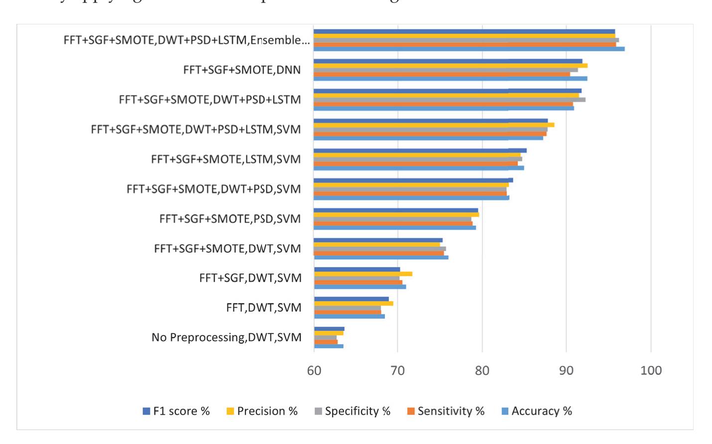
**Figure 12.** Comparison of results achieved for consumer choice recognition by using different experiments.
Different experiments were conducted and different kinds of feature-extraction techniques were applied. In first iteration, the features were extracted by using DWT, and experimental settings for preprocessing and classification was the same as previous experiments. By analyzing the results, it was concluded that there is no such improvement in accuracy, specificity, sensitivity, precision, or F1 score. Consequently, concatenation of the DWT and PSD featues was performed, and then the signals were classified in terms of
124
*Sensors* **2022**, *22*, 9744
likes and dislikes and came to know that there was improvement in the results. For the next iteration, we have concatenated DWT-, PSD-, and LSTM-based features and compiled the results.The results show that there is a significant amount of improvement in accuracy, specificity, sensitivity, precision, and F1 score by the concatenation of handcrafted features with automated features by LSTM.
In the last experiment, the experimental settings for preprocessing and feature extraction are the same, and classification was iterated by using different classifiers like DNN, SVM, and decision tree. The highest accuracy achieved was 92.68%, which was not acceptable, so the ensemble classifier was employed. The weights for each classifier were passed to the genetic algorithm for optimization. The highest accuracy achieved is 96.89%, with specificity of 96.21% , sensitivity of 95.89%, precision of 95.78%, and F1 score of 95.76%.
Figure 13 shows us the comparison of the confusion matrix for consumer emotion prediction.
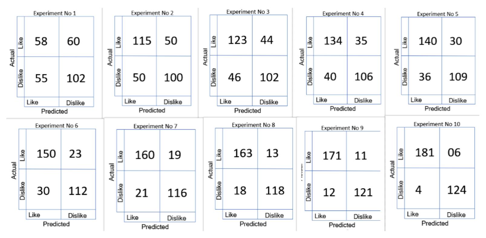
**Figure 13.** Comparison of confusion matrix for different experimental settings.
#### 11. Evaluation of the Effectiveness of the Proposed Method in Comparison to State-of-the-Art Customer Choice Recognition Systems
A dataset consisting of electroencephalogram readings was employed in order to make a comparison between the results obtained by the proposed method and those obtained by traditional consumer choice recognition techniques. The performance of the proposed approach is superior compared to the existing methods.The system for recognizing consumer choice can be adversely affected by an increase in sensitivity with low specificity. The accuracy is 88%, but specificity is 86.76%, which reveals the high false alarm rate that affects the recognition of consumer choice negatively [13]. It is possible to detect the consumer preference on various e-commerce products; however, Jafar et al. [65] were unable to obtain sensitivity and specificity greater than 69%. Aldayel et al. [4] suggested a consumer choice recognition system with an average sensitivity of 91.2%, but only 81.5% specificity. Rupali et al. [57] and Yadava et al. [1] have employed DWT for feature extraction, but the proposed architecture uses automated as well as handcrafted characteristics to classify between likes and dislikes. The proposed method has obtained a sensitivity of 95.89% while maintaining a specificity of 96.21%. The results of the suggested technique are compared with recent state-of-the-art methodologies in Table 7, which examines the three concepts of accuracy, specificity, and sensitivity.
125
*Sensors* **2022**, *22*, 9744
**Table 7.** Comparison of different state of the art customer choice recognition systems.
| Method | Preprocessing | Features | Classifier | Accuracy | Sensitivity | Specificity |
|------------------------------------|------------------------------------------------|----------------------|-------------------------|----------|-------------|-------------|
| Amna et al. [13] (2022) | Savitzky–Golay Filter | - | Boosted Tree Classifier | 88.89% | 84.68% | 86.76% |
| Abeer al Nafjan et al. [54] (2022) | bandpass Filter | PCA | DNN | 94% | - | - |
| P.Santhiya et al. [55] (2022) | ICA | NW-STFT | SVM | 91% | 90.23% | 89.97% |
| Somayeh et al. [56] (2022) | ICA | PSD | Statistical Analysis | 93% | - | - |
| Rupali et al. [57] (2021) | bandpass Filter | DWT | LSTM | 92% | 90.36% | 91.86% |
| Adam et al. [14] (2021) | Notch Filter | PCA | SVM, KNN | 68.50% | - | - |
| Aldayel et al. [4] (2021) | Bandpass Filter | DWT | DNN | 87% | 91.2 | 81.5 |
| Yilmaz et al. [58] (2018) | bandpass Filter | Statistical Features | SVM | 82.55% | 78.63% | 80.79% |
| Jafar et al [20] (2018) | - | Statistical Features | Decision Tree | 68.33% | 67.98% | 66.37% |
| Yadava et al [1] (2017) | Savitzky-Golay Filter | DWT | HMM | 70% | - | - |
| Teo et al. [17] (2017) | - | DNN | DNN | 74.60% | 71.49% | 73.60% |
| Chew et al. [15] (2016) | Average Filter | PSD | SVM | 80% | 82.3 | 80.5 |
| Maarten et al. [59] (2015) | -, ICA | FFT | SVM | 68% | - | - |
| Hakim et al. [52] (2015) | - | Statistical Analysis | DT | 68.50% | - | - |
| Ariel et al. [8] (2013) | Low Pass Filter | Statistical Features | Cardinal Analysis | 65% | 61.73% | 64.19% |
| Proposed Method | Bandpass Filter, Savitzkay Golay Filter, SMOTE | LSTM, DWT, PSD | Ensemble Classifier | 96.89% | 95.89% | 96.21% |
The ROC curve is another crucial efficiency metric. This graph shows how well a classification system performs in terms of sensitivity versus the percentage of false positives. This experimental setting comprises the preprocessing of EEG signals by applying bandpass filtering, FFT, SMOTE, and the Savitzky–Golay filter, as well as the feature extraction and categorization of extensive feature set by using an ensemble classifier. It has been discovered that the method that was proposed is capable of reaching better sensitivity while keeping a low number of false positives. The outcomes of the proposed system are compared with those of the state-of-the-art systems in Table 7. The proposed system has higher levels of both specificity and sensitivity. Therefore, it is crucial to get a high, genuinely positive rate and low false positives by having a class with a high degree of similarity chosen as the positive class. According to the findings, the proposed system outperforms the state of the art in terms of both true positive rates and false positives.
#### 12. Conclusions and Future Directions
The first phase in consumer choice recognition often involves the preprocessing of EEG signals, followed by feature extraction and classification. Numerous academics have attempted to forecast customer preferences in terms of likes and dislikes during the past few years. The procedure of gauging customer choice with greater sensitivity and specificity has proven difficult. Effective preprocessing of EEG signals includes removing EEG signals' noise from EEG signals and to deal with the problem of class imbalance caused by fewer data samples from the like class in comparison with the dislike class and extracting features that give high interclass variance to assist in accurate classification of like and dislike states are some of the issues that must be resolved. Researchers have not been able to enhance classification accuracy without preprocessing of EEG signals; hence, preprocessing and noise removal plays a critical role in attaining improved accuracy. Researchers have adopted the notch, Butterworth, PCA, and ICA for the preprocessing of EEG signals. However, the results reveal that FFT, SMOTE, and bandpass filter do a better job of boosting the SNR than other approaches.
In recent studies researchers used PSD to extract features, whereas decision tree was used for classification. To improve the performance evaluation metrics like accuracy, specificity, and sensitivity, the proposed model was tested by using different classifiers, but the improved accuracy, sensitivity, and specifivity was achieved by an ensemble classifier that classifies the EEG signals by optimizing the weights of classifiers like DNN, SVM, and RF by genetic algorithm. Several gaps were determined in preprocessing and feature extraction after conducting this comparison. Feature extraction implies a customized LSTM architecture. The sensitivity and specificity of these approaches have been assessed. In
126
*Sensors* **2022**, *22*, 9744
the existing systems, the problem of class imbalance was not confronted. In the proposed method to deal with class imbalance, the SMOTE technique was employed.
The proposed method makes use of SMOTE to generate like class samples to resolve the problem of class imbalance. For classification of EEG signals, we employed different classifiers but could not achieve the desired accuracy. Consequently, an ensemble classifier was employed, and weights from different classifiers were optimized by using the genetic algorithm. It is significant that our proposed technique has improved sensitivity, specificity, accuracy, precision, and F1 score. In this dataset, three performance indicators have yet to be attained by any existing methods. According to the results, our proposed method's ROC curve assessment outperforms existing methods in terms of increased sensitivity and specificity. In the future, we can also employ generative adversarial networks (GANs) for synthetic data generation. It is possible that future research will examine different techniques to deal with fake responses. Furthermore, a neutral choice for the products might be implemented to present users with more options. When viewing products, the tracking of a user's eye movement could be seen as additional parameter in the prediction of preferred choices. To improve the prediction outcomes, it may be necessary to investigate more robust features and classifier combinations. Secondly, for good results we can also focus on the dataset. In this research, the total instances for our ensemble classifier are 1050, which could be considered a small number of examples. Consequently, in the future we can apply our model to the dataset having large instances of customer preferences to obtain better results.
**Author Contributions:** Formal analysis, W.M.; Investigation, H.E. and A.D.A.; Writing—original draft, S.M.A.S., S.M.U., S.K., I.U.R., A.A., S.H. and S.S.U. All authors have read and agreed to the published version of the manuscript.
**Funding:** This research was funded by Princess Nourah bint Abdulrahman University Researchers Supporting Project number (PNURSP2022R51), Princess Nourah bint Abdulrahman University, Riyadh, Saudi Arabia.
**Institutional Review Board Statement:** Not applicable.
**Informed Consent Statement:** Not applicable.
**Data Availability Statement:** Not applicable.
**Acknowledgments:** The authors would like to acknowledge Princess Nourah bint Abdulrahman University Researchers Supporting Project number (PNURSP2022R51), Princess Nourah bint Abdulrahman University, Riyadh, Saudi Arabia.
**Conflicts of Interest:** The authors declare no conflict of interest.
#### References
- 1. Aldayel, M.; Ykhlef, M.; Al-Nafjan, A. Recognition of consumer preference by analysis and classification EEG signals. *Front. Hum. Neurosci.* **2021**, *14*, 604639. [CrossRef] [PubMed]
- 2. Yadava, M.; Kumar, P.; Saini, R.; Roy, P.P.; Prosad Dogra, D. Analysis of EEG signals and its application to neuromarketing. *Multimed. Tools Appl.* **2017**, *76*, 19087–19111. [CrossRef]
- 3. Shao, G.N.; Kim, H.; Imran, S. 2016 Use of EEG for Neuromarketing Applications. Available online: https://www.sciencedirect. com/science/article/abs/pii/S092633731500346X (accessed on 5 September 2021).
- 4. Aldayel, M.; Ykhlef, M.; Al-Nafjan, A. Deep learning for EEG-based preference classification in neuromarketing. *Appl. Sci.* **2020**, *10*, 1525. [CrossRef]
- 5. Hammou, K.A.; Galib, M.H.; Melloul, J. The contributions of neuromarketing in marketing research. *J. Manag. Res.* **2013**, *5*, 20.
- 6. Lin, M.H.J.; Cross, S.N.; Jones, W.J.; Childers, T.L. Applying EEG in consumer neuroscience. *Eur. J. Mark.* **2018**, *52*, 66–91. [CrossRef]
- 7. Telpaz, A.; Webb, R.; Levy, D.J. Using EEG to predict consumers' future choices. *J. Mark. Res.* **2015**, *52*, 511–529. [CrossRef]
- 8. Hwang, H.J.; Kim, S.; Choi, S.; Im, C.H. EEG-based brain-computer interfaces: A thorough literature survey. *Int. J. Hum.-Comput. Interact.* **2013**, *29*, 814–826. [CrossRef]
- 9. Al-Fahoum, A.S.; Al-Fraihat, A.A. Methods of EEG signal features extraction using linear analysis in frequency and time-frequency domains. *Int. Sch. Res. Not.* **2014**, *2014*, 730218. [CrossRef]
127
*Sensors* **2022**, *22*, 9744
- 10. Chew, L.H.; Teo, J.; Mountstephens, J. Aesthetic preference recognition of 3D shapes using EEG. *Cogn. Neurodyn.* **2016**, *10*, 165–173. [CrossRef]
- 11. Alharithi, F.S.; Almulihi, A.H.; Bourouis, S.; Alroobaea, R.; Bouguila, N. Discriminative Learning Approach Based on Flexible Mixture Model for Medical Data Categorization and Recognition. *Sensors* **2021**, *21*, 2450. [CrossRef]
- 12. Abdulkader, S.N.; Atia, A.; Mostafa, M.S.M. Brain computer interfacing: Applications and challenges. *Egypt. Inform. J.* **2015**, *16*, 213–230. [CrossRef]
- 13. Khan, A.; Rasool, S. Game induced emotion analysis using electroencephalography. *Comput. Biol. Med.* **2022**, *145*, 105441. [CrossRef] [PubMed]
- 14. Almulihi, A.H.; Alharithi, F.S.; Bourouis, S.; Alroobaea, R.; Pawar, Y.; Bouguila, N. Oil Spill Detection in SAR Images Using Online Extended Variational Learning of Dirichlet Process Mixtures of Gamma Distributions. *Remote Sens.* **2021**, *13*, 2991. [CrossRef]
- 15. Bazzani, A.; Ravaioli, S.; Faraguna, U.; Turchetti, G. Is EEG suitable for marketing research? A systematic review. *Front. Neurosci.* **2020**, *14*, 1343. [CrossRef] [PubMed]
- 16. Gauba, H.; Kumar, P.; Roy, P.P.; Singh, P.; Dogra, D.P.; Raman, B. Prediction of advertisement preference by fusing EEG response and sentiment analysis. *Neural Netw.* **2017**, *92*, 77–88. [CrossRef] [PubMed]
- 17. Teo, J.; Hou, C.L.; Mountstephens, J. Deep learning for EEG-Based preference classification. *Aip Conf. Proc.* **2017**, *1891*, 020141.
- 18. Devaru, S.D.B. Significance of Neuromarketing on consumer buying behaviour. *Int. J. Tech. Res. Sci. SIGNIFICANCE* **2018**, *3*, 114–121.
- 19. Yilmaz, B.; Korkmaz, S.; Arslan, D.B.; Güngör, E.; Asyalı, M.H. Like/dislike analysis using EEG: Determination of most discriminative channels and frequencies. *Comput. Methods Programs Biomed.* **2014**, *113*, 705–713. [CrossRef]
- 20. Zamani, J.; Naieni, A.B. Best Feature Extraction and Classification Algorithms for EEG Signals in Neuromarketing. *Front. Biomed. Technol.* **2020**, *7*, 186–191. [CrossRef]
- 21. Bastiaansen, M.; Straatman, S.; Driessen, E.; Mitas, O.; Stekelenburg, J.; Wang, L. My destination in your brain: A novel neuromarketing approach for evaluating the effectiveness of destination marketing. *J. Destin. Mark. Manag.* **2018**, *7*, 76–88. [CrossRef]
- 22. Khushaba, R.N.; Wise, C.; Kodagoda, S.; Louviere, J.; Kahn, B.E.; Townsend, C. Consumer neuroscience: Assessing the brain response to marketing stimuli using electroencephalogram (EEG) and eye tracking. *Expert Syst. Appl.* **2013**, *40*, 3803–3812. [CrossRef]
- 23. Kawasaki, M.; Yamaguchi, Y. Effects of subjective preference of colors on attention-related occipital theta oscillations. *NeuroImage* **2012**, *59*, 808–814. [CrossRef] [PubMed]
- 24. Ohme, R.; Reykowska, D.; Wiener, D.; Choromanska, A. Application of frontal EEG asymmetry to advertising research. *J. Econ. Psychol.* **2010**, *31*, 785–793. [CrossRef]
- 25. Usman, S.M.; Khalid, S.; Akhtar, R.; Bortolotto, Z.; Bashir, Z.; Qiu, H. Using scalp EEG and intracranial EEG signals for predicting epileptic seizures: Review of available methodologies. *Seizure* **2019**, *71*, 258–269. [CrossRef] [PubMed]
- 26. Guo, G.; Elgendi, M. A new recommender system for 3D e-commerce: An EEG based approach. *J. Adv. Manag. Sci.* **2013**, *1*, 61–65. [CrossRef]
- 27. Morin, C. Neuromarketing: The new science of consumer behavior. *Society* **2011**, *48*, 131–135. [CrossRef]
- 28. Vecchiato, G.; Fallani, F.D.V.; Astolfi, L.; Toppi, J.; Cincotti, F.; Mattia, D.; Salinari, S.; Babiloni, F. The issue of multiple univariate comparisons in the context of neuroelectric brain mapping: An application in a neuromarketing experiment. *J. Neurosci. Methods* **2010**, *191*, 283–289. [CrossRef]
- 29. Khushaba, R.N.; Greenacre, L.; Kodagoda, S.; Louviere, J.; Burke, S.; Dissanayake, G. Choice modeling and the brain: A study on the Electroencephalogram (EEG) of preferences. *Expert Syst. Appl.* **2012**, *39*, 12378–12388. . [CrossRef]
- 30. Usman, S.M.; Khalid, S.; Aslam, M.H. Epileptic seizures prediction using deep learning techniques. *IEEE Access* **2020**, *8*, 39998–40007. [CrossRef]
- 31. Usman, S.M.; Khalid, S.; Bashir, Z. Epileptic seizure prediction using scalp electroencephalogram signals. *Biocybern. Biomed. Eng.* **2021**, *41*, 211–220. [CrossRef]
- 32. Jirayucharoensak, S.; Pan-Ngum, S.; Israsena, P. EEG-based emotion recognition using deep learning network with principal component based covariate shift adaptation. *Sci. World J.* **2014**, *2014*, 627892. [CrossRef] [PubMed]
- 33. Bashivan, P.; Rish, I.; Yeasin, M.; Codella, N. Learning representations from EEG with deep recurrent-convolutional neural networks. *arXiv* **2015**, arXiv:1511.06448.
- 34. Zhang, D.; Yao, L.; Zhang, X.; Wang, S.; Chen, W.; Boots, R. EEG-based intention recognition from spatio-temporal representations via cascade and parallel convolutional recurrent neural networks. *arXiv* **2017**, arXiv:1708.06578.
- 35. Schirrmeister, R.T.; Springenberg, J.T.; Fiederer, L.D.J.; Glasstetter, M.; Eggensperger, K.; Tangermann, M.; Hutter, F.; Burgard, W.; Ball, T. Deep learning with convolutional neural networks for EEG decoding and visualization. *Hum. Brain Mapp.* **2017**, *38*, 5391–5420. [CrossRef] [PubMed]
- 36. Xun, G.; Jia, X.; Zhang, A. Detecting epileptic seizures with electroencephalogram via a context-learning model. *BMC Med. Inform. Decis. Mak.* **2016**, *16*, 97–109. [CrossRef]
- 37. Hasanin, T.; Khoshgoftaar, T.M.; Leevy, J.L.; Bauder, R.A. Severely imbalanced big data challenges: Investigating data sampling approaches. *J. Big Data* **2019**, *6*, 1–25. [CrossRef]
128
*Sensors* **2022**, *22*, 9744
- 38. Khan, M.Z.; Naseem, R.; Anwar, A.; Haq, I.U.; Alturki, A.; Ullah, S.S.; Al-Hadhrami, S.A. A novel approach to automate complex software modularization using a fact extraction system. *J. Math.* **2022**, *2022*, 8640596. [CrossRef]
- 39. Usman, S.M.; Khalid, S.; Bashir, S. A deep learning based ensemble learning method for epileptic seizure prediction. *Comput. Biol. Med.* **2021**, *136*, 104710. [CrossRef]
- 40. Usman, S.M.; Khalid, S.; Jabbar, S.; Bashir, S. Detection of preictal state in epileptic seizures using ensemble classifier. *Epilepsy Res.* **2021**, *178*, 106818. [CrossRef]
- 41. Ren, Y.; Wu, Y. Convolutional deep belief networks for feature extraction of EEG signal. In Proceedings of the IEEE 2014 International Joint Conference on Neural Networks (IJCNN), Beijing, China, 6–11 July 2014; pp. 2850–2853.
- 42. Ioannides, A.A.; Liu, L.; Theofilou, D.; Dammers, J.; Burne, T.; Ambler, T.; Rose, S. Real time processing of affective and cognitive stimuli in the human brain extracted from MEG signals. *Brain Topogr.* **2000**, *13*, 11–19. [CrossRef]
- 43. Ambler, T.; Ioannides, A.; Rose, S. Brands on the brain: Neuro-images of advertising. *Bus. Strategy Rev.* **2000**, *11*, 17–30. [CrossRef]
- 44. Chakravarthi, B.; Ng, S.C.; Ezilarasan, M.; Leung, M.F. EEG-based emotion recognition using hybrid CNN and LSTM classification. *Front. Comput. Neurosci.* **2022**.
- 45. Dmochowski, J.P.; Bezdek, M.A.; Abelson, B.P.; Johnson, J.S.; Schumacher, E.H.; Parra, L.C. Audience preferences are predicted by temporal reliability of neural processing. *Nat. Commun.* **2014**, *5*, 1–9. [CrossRef] [PubMed]
- 46. Braeutigam, S.; Rose, S.P.; Swithenby, S.J.; Ambler, T. The distributed neuronal systems supporting choice-making in real-life situations: Differences between men and women when choosing groceries detected using magnetoencephalography. *Eur. J. Neurosci.* **2004**, *20*, 293–302. [CrossRef] [PubMed]
- 47. Senior, C. Beauty in the brain of the beholder. *Neuron* **2003**, *38*, 525–528. [CrossRef] [PubMed]
- 48. Gupta, A.; Shreyam, R.; Garg, R.; Sayed, T. Correlation of neuromarketing to neurology. In Proceedings of the International Conference on Materials, Alloys and Experimental Mechanics (ICMAEM-2017), Narsimha Reddy Engineering College, Hyderabad, India, 3–4 July 2017; Volume 225, p. 012129.
- 49. Reddy, G.T.; Bhattacharya, S.; Ramakrishnan, S.S.; Chowdhary, C.L.; Hakak, S.; Kaluri, R.; Reddy, M.P.K. An ensemble based machine learning model for diabetic retinopathy classification. In Proceedings of the 2020 International Conference on Emerging Trends in Information Technology and Engineering (ic-ETITE), Vellore, India, 24–25 February 2020; pp. 1–6.
- 50. Murugappan, M.; Murugappan, S.; Gerard, C. Wireless EEG signals based neuromarketing system using Fast Fourier Transform (FFT). In Proceedings of the 2014 IEEE 10th International Colloquium on Signal Processing and Its Applications, Kuala Lumpur, Malaysia, 7–9 March 2014; pp. 25–30.
- 51. McClure, S.M.; Li, J.; Tomlin, D.; Cypert, K.S.; Montague, L.M.; Montague, P.R. Neural correlates of behavioral preference for culturally familiar drinks. *Neuron* **2004**, *44*, 379–387. [CrossRef]
- 52. Savitzky, A.; Golay, M.J. Smoothing and differentiation of data by simplified least squares procedures. *Anal. Chem.* **1964**, *36*, 1627–1639. [CrossRef]
- 53. Haq, I.U.; Anwar, A.; Basharat, I.; Sultan, K. Intelligent tutoring supported collaborative learning (ITSCL): A hybrid framework. *Int. J. Adv. Comput. Sci. Appl.* **2020**, *11*, 523–535. [CrossRef]
- 54. Al-Nafjan, A. Feature selection of EEG signals in neuromarketing. *PeerJ Comput. Sci.* **2022**, *8*, e944. [CrossRef]
- 55. Santhiya, P.; Chitrakala, S. PTCERE: Personality-trait mapping using cognitive-based emotion recognition from electroencephalogram signals. *Vis. Comput.* **2022**. [CrossRef]
- 56. Raiesdana, S.; Mousakhani, M. An EEG-Based Neuromarketing Approach for Analyzing the Preference of an Electric Car. *Comput. Intell. Neurosci.* **2022**, *2022*, 9002101. [CrossRef] [PubMed]
- 57. Gill, R.; Singh, J. A Proposed LSTM-Based Neuromarketing Model for Consumer Emotional State Evaluation Using EEG. *Adv. Anal. Deep. Learn. Model.* **2022**. [CrossRef]
- 58. Adam, H.; Klorfeld, S.; Sela, T.; Friedman, D.; Shabat-Simon, M.; Levy, D.J. Machines learn neuromarketing: Improving preference prediction from self-reports using multiple EEG measures and machine learning. *Int. J. Res. Mark.* **2021**, *38*, 770–791.
- 59. Murugappan, M.; Ramachandran, N.; Sazali, Y. Classification of human emotion from EEG using discrete wavelet transform. *J. Biomed. Sci. Eng.* **2010**, *3*, 390. [CrossRef]
- 60. Nilashi, M.; Samad, S.; Ahmadi, N.; Ahani, A.; Abumalloh, R.A.; Asadi, S.; Abdullah, R.; Ibrahim, O.; Yadegaridehkordi, E. Neuromarketing: A review of research and implications for marketing. *J. Soft Comput. Decis. Support Syst.* **2020**, *7*, 23–31.
- 61. Shaabani, M.; Fuad, N.; Jamal, N.; Ismail, M. kNN and SVM classification for EEG: A review. *InECCE2019* **2020**, *632*, 555–565.
- 62. Kang, J.; Han, X.; Song, J.; Niu, Z.; Li, X. The identification of children with autism spectrum disorder by SVM approach on EEG and eye-tracking data. *Comput. Biol. Med.* **2020**, *120*, 103722. [CrossRef]
- 63. Bourouis, S.; Bouguila, N. Nonparametric learning approach based on infinite flexible mixture model and its application to medical data analysis. *Int. J. Imaging Syst. Technol.* **2021**, *31*, 1989–2002. [CrossRef]
- 64. Hadjidimitriou, S.K.; Hadjileontiadis, L.J. Toward an EEG-based recognition of music liking using time-frequency analysis. *IEEE Trans. Biomed. Eng.* **2012**, *59*, 3498–3510. [CrossRef]
- 65. Rakshit, A.; Lahiri, R. Discriminating different color from EEG signals using interval-type 2 fuzzy space classifier (a neuromarketing study on the effect of color to Cognitive State). In Proceedings of the 2016 IEEE 1st International Conference on Power Electronics, Intelligent Control and Energy Systems (ICPEICES), Delhi, India, 4–6 July 2016; pp. 1–6.
129


*Article*
### Electroencephalography Reflects User Satisfaction in Controlling Robot Hand through Electromyographic Signals
**Hyeonseok Kim 1, Makoto Miyakoshi 1, Yeongdae Kim 2, Sorawit Stapornchaisit 3, Natsue Yoshimura 4 and Yasuharu Koike 4,\***
- 1 Swartz Center for Computational Neuroscience, Institute for Neural Computation, University of California San Diego, La Jolla, CA 92093, USA
- 2 Department of Industrial Engineering and Economics, Tokyo Institute of Technology, Tokyo 152-8550, Japan
- 3 Department of Information and Communications Engineering, Tokyo Institute of Technology, Yokohama 226-0026, Japan
- 4 Institute of Innovative Research, Tokyo Institute of Technology, Yokohama 226-0026, Japan
- **\*** Correspondence: koike@pi.titech.ac.jp
**Abstract:** This study addresses time intervals during robot control that dominate user satisfaction and factors of robot movement that induce satisfaction. We designed a robot control system using electromyography signals. In each trial, participants were exposed to different experiences as the cutoff frequencies of a low-pass filter were changed. The participants attempted to grab a bottle by controlling a robot. They were asked to evaluate four indicators (stability, imitation, response time, and movement speed) and indicate their satisfaction at the end of each trial by completing a questionnaire. The electroencephalography signals of the participants were recorded while they controlled the robot and responded to the questionnaire. Two independent component clusters in the precuneus and postcentral gyrus were the most sensitive to subjective evaluations. For the moment that dominated satisfaction, we observed that brain activity exhibited significant differences in satisfaction not immediately after feeding an input but during the later stage. The other indicators exhibited independently significant patterns in event-related spectral perturbations. Comparing these indicators in a low-frequency band related to the satisfaction with imitation and movement speed, which had significant differences, revealed that imitation covered significant intervals in satisfaction. This implies that imitation was the most important contributing factor among the four indicators. Our results reveal that regardless of subjective satisfaction, objective performance evaluation might more fully reflect user satisfaction.
**Keywords:** electromyography; electroencephalography; satisfaction; subjective response; robot control
Academic Editors: Yifan Zhao, Fei He and Yuzhu Guo
Received: 22 November 2022 Revised: 23 December 2022 Accepted: 25 December 2022 Published: 27 December 2022

**Copyright:** © 2022 by the authors. Licensee MDPI, Basel, Switzerland. This article is an open access article distributed under the terms and conditions of the Creative Commons Attribution (CC BY) license (https:// creativecommons.org/licenses/by/ 4.0/).
### 1. Introduction
In the development of an advanced human–robot interface, user satisfaction should be investigated to determine the optimal control configuration. Several studies have evaluated interface usability [1–3] and user satisfaction [4]. For an individualized interface, the system must recognize the reactions of the user to its responses. Although some studies have investigated brain-related user responses, such as brain activity reflecting delayed response during real-time cursor control [5], brain activity during control for interfacing has rarely been investigated regarding subjective feelings. Brain activity related to a variety of subjective feelings has been investigated based on self-reported information. For example, brain activity with respect to changes due to the mood of a film was investigated in [6]. Changes in emotional states induced by auditory stimuli were investigated using electroencephalogram (EEG) signals [7], and emotional states related to music were investigated using EEG data [8]. The use of EEG signals to detect emotion has been validated by several classification methods such as support vector machine, k-nearest neighbor, naive Bayes, long- and short-term memory, and deep belief networks (DBNs) [9]. In addition, *Sensors* **2023**, *23*, 277. https://doi.org/10.3390/s23010277 https://www.mdpi.com/journal/sensors
130
*Sensors* **2023**, *23*, 277
because EEG signals have been involved in a variety of analysis methods, such as fuzzy decision tree [10], and combined with other sensors [11], they can be adopted for subjective evaluation of human–robot interfaces.
Users control a robot for a purpose (e.g., to grasp an object). If they fail to control the robot or feel that it might not grasp the object, they feed a different input into the robot. In such cases, when a user gives up or succeeds in moving the robot, defining the user's satisfaction in a trial is necessary. To track the source of the satisfaction, first, we need to understand the moment that dominates the satisfaction and the factors of robot movement that induce user satisfaction. The representation of objective indicators of robot movement by the brain has not been elucidated. This could be linked to the user's evaluation of the robotic performance, which is information that could be exploited.
However, the timing of and the factors that affect satisfaction remain unclear. Satisfaction can be measured by subjective responses to a questionnaire. We attempted to determine brain activity related to satisfaction and the important interval, which dominates satisfaction, according to the difference between EEG in unsatisfactory and satisfactory tasks. For factors that cause satisfaction, we selected four indicators (stability, imitation, response time, and movement speed) related to the robot's performance to determine the extent to which these performance-related indicators, which might be independent of satisfaction, are relevant to satisfaction. We categorized performance indicators as abstract and direct indicators. By determining parameters that the robot system can handle, we can focus on the parameters of satisfaction. Otherwise, we should determine abstract concepts for performance evaluation that primarily contribute to satisfaction within the brain. However, if we cannot use abstract parameters for robot control, they can be decomposed for easy handling. Unlike speed and time, stability and imitation were intended to represent abstract indicators. This enables us to determine whether satisfaction can be attributed to directly controllable indicators. The subjective responses obtained from the questionnaire can be linked to EEG signals to determine relevant brain areas and are observed in the same region as satisfaction.
This study investigated aspects of both satisfaction and EMG-based robotic control. We designed a system controlled by EMG signals. In each trial, we exposed the participants to different experiences by changing the cutoff frequencies (1, 2, 5, and 10 Hz) of a lowpass filter for the input EMG signals. The participants attempted to grab a bottle by controlling the robot. At the end of each trial, the participants were asked to complete a questionnaire to evaluate the four indicators and their satisfaction levels. The EEG signals of the participants were recorded while they controlled the robot and responded to the questionnaire. We further compared the brain activities based on five parameters (the aforementioned four indicators and the level of satisfaction).
#### 2. Experimental Procedures
#### 2.1. Participants
A group of eight healthy individuals comprising five men and three women participated in the experiment. The mean and standard deviation of their ages were 26.75 years and 3.33 years, respectively. All participants were right-handed and provided written informed consent before the experiment. This study was conducted as per the Declaration of Helsinki and approved by the ethics committee of the Tokyo Institute of Technology (ethics number: 2019002).
#### 2.2. Experimental Apparatus and Data Collection
Figure 1 shows the experimental environment. A controllable robotic hand (qb Soft-Hand, qbrobotics, Navacchio, Italy) was fixed in front of a table. The robot provides 19 anthropomorphic DOFs, one synergy, one motor, 1.7 kg of nominal payload, 0.77 kg of weight, and 1.1 s for clenched fists from a wide-open position. The bottle was placed near the robotic hand. During the experiment, the participants sat on a chair and wore an EEG cap. The sitting posture enabled them to see the robotic hand and screen. Their
131
*Sensors* **2023**, *23*, 277
left hand was placed on a keyboard to answer the questionnaire, and their right arm was placed on an armrest. To fix an EMG sensor, an arm brace was worn on their right hand. In addition, the participants wore a face cover with opaque paper, which prevented them from seeing their right hand. EMG signals from 32 channels were measured with an array EMG sensor [12] and 24 bit resolution at a sampling rate of 500 Hz and used for robotic control. An OptiTrack motion capture system (NaturalPoint, Inc., Corvallis, OR, USA) recorded the motions of the participants and robotic hand. Three motion capture markers were attached to the back of the wrist on the end of the radius/ulna, back of the hand on the third metacarpal bone, and back of the middle finger (between the metacarpophalangeal and proximal interphalangeal joints) of the participants and the robot. EEG signals were recorded from 64 electrodes using a BioSemi ActiveTwo system (BioSemi, Amsterdam, Netherlands) with 24 bit resolution at a sampling rate of 512 Hz, as shown in Table 1.
**Figure 1.** Experimental environment (not to scale). During the experiment, participants sat on a chair and placed their right arm on an armrest attached to the table. A keyboard was placed on the table through which participants responded to questions by pressing a button. For the task, participants were asked to grab a bottle, which was positioned such that the robot hand could be bent to grab the bottle. The robot hand could bend/extend a wrist and grip fingers with one degree of freedom (DOF). An opaque face cover prevented the participants from seeing their right arm. A monitor was placed in front of the table along the midline of the body, which includes a robot hand on the line to enable participants to easily see the screen.
132
*Sensors* **2023**, *23*, 277
**Table 1.** Electrodes and description of electrode labels.
| Label | Meaning |
|-----------------------------|-------------------------------------------------------------------------------------------------------------------------------------------------------------------------------------------------------------------------------------------------------------------------------------------------------------------|
| Fp | Prefrontal lobe |
| F | Frontal lobe |
| T | Temporal lobe |
| P | Parietal lobe |
| O | Occipital lobe |
| C | Central lobe |
| Combination of above labels | Position between two places |
| Even numbers | The right hemisphere |
| Odd numbers | The left hemisphere |
| Z | The midline on the coronal plane |
| Used electrodes | Fp1, Fp2, Fpz, AF3, AF4, AF7, AF8, AFz, F1, F2, F3,
F4, F5, F6, F7, F8, Fz, FT7, FT8, FC1, FC2, FC3, FC4,
FC5, FC6, FCz, C1, C2, C3, C4, C5, C6, Cz, T7, T8,
TP7, TP8, CP1, CP2, CP3, CP4, CP5, CP6, CPz, P1,
P2, P3, P4, P5, P6, P7, P8, P9, P10, Pz, PO3, PO4,
PO7, PO8, POz, O1, O2, Oz, and Iz |
#### 2.3. Experimental Paradigm
Calibration was necessary because the robotic hand was controlled using only EMG signals. First, each participant sat on a chair and placed their right arm on the armrest, as shown in Figure 1. Then, they were instructed to perform six different hand motions: hand gripping/opening, wrist flexion/extension, and pronation/supination. Each hand motion was repeated thrice. The EMG signals measured during the motions were rectified and filtered with a second-order Butterworth low-pass filter with a cutoff frequency of 5 Hz. Noisy channels were rejected before preprocessing. By using the hierarchical alternating least squares algorithm [13], we extracted two muscle synergies from the EMG signals involved in the gripping/opening motions and four muscle synergies from those involved in the other motions. If the extracted muscle synergies did not reflect the expected movement, the number of synergies was increased. The weight of each muscle synergy was normalized to the maximum weight. Next, the joint angles were estimated using a musculoskeletal model [14] and introduced into the robot hand as an input command. After calibration, the participants learned to control the robot hand. They were subsequently instructed to remember and replicate their methods of controlling the robot hand during the task. However, if a participant failed to control the robot, the calibration process was repeated.
In the experiment, we used four cutoff frequencies (1, 2, 5, and 10 Hz) of the low-pass filter of the EMG signals. The participants were exposed to different control experiences. Each trial had one of the four cutoff frequencies, which were determined randomly. The participants were not informed of the aspects that were changed or the various options available. They were only informed that they would have different control experiences in each trial. At the beginning of the experiment, a "wait" message appeared on the screen, and the participants immediately put their hands in a resting state. When the message was changed to "Go", the participants attempted to grab the bottle by controlling the robot. This was achieved by flexing their wrists and grasping their hands. When the robot hand approached the bottle tracked by motion capture markers, a questionnaire appeared on the screen after 2 s. However, this information was concealed from the participants. Notably, no trial in which the interval between the "Go" cue and the questionnaire was less than 2 s occurred. The participants were asked to evaluate the following four indicators related to the control performance: stability (unstable vs. stable), imitation (bad vs. good), response time (delay vs. no delay), and movement speed (extremely slow vs. extremely
133
*Sensors* **2023**, *23*, 277
fast). Stability and imitation were selected as more abstract indicators than speed and time to determine whether satisfaction was attributed to directly controllable indicators. After answering the survey, they were asked to evaluate their subjective satisfaction, regardless of the objective performance of the robot. The questionnaire was designed using a five-point Likert scale. When they completed the questionnaires, a "relax" message appeared on the screen until the next trial began. This procedure was subsequently repeated. The indicators are defined as follows: stability refers to the extent to which the robot shakes unnecessarily or performs unnecessary movement during the trial, imitation is determined by the extent to which the robot's movement is identical to the movement of the actual hand, response time refers to the time required to move the robot, movement speed is determined by the speed of the robot during the trial, and satisfaction is determined by the extent of the participants' feelings about the trial if they used this interface as a user.
The participants were required to perform three runs, with each run consisting of 81 trials and a break between successive runs. For each run, a frequency of 10 Hz was presented 21 times, and the other frequencies were presented 20 times each. Participant 6 performed two runs, and participant 1 performed one run consisting of 97 trials (25 trials for the 10 Hz and 24 trials for each of the others).
#### 2.4. EEG Analysis
EEGLAB was used for preprocessing [15] as follows: EEG data were resampled at a frequency of 256 Hz and filtered using a high-pass filter with a cutoff frequency of 1 Hz. We used cleanLineNoise [16] to remove line noise and artifact subspace reconstruction (ASR) to correct the artifacts [17,18]. The cutoff parameter for the ASR was set to 10. Cleaned data were re-referenced to the average. Next, we performed an independent component analysis using Adaptive Mixture ICA. An equivalent dipole model corresponding to each independent component was fitted using fitTwoDipole [19]. All independent components were identified using ICLabel [20].
The components identified as the brain were used for group-level analysis, for which k-means clustering was performed based on the dipole locations of the brain components. Ten clusters were determined using the silhouette index [21]. We extracted epochs between 0 s ("Go" cue) and 2 s after the "Go" cue to calculate the event-related spectral perturbations (ERSPs) of the independent components within a frequency of 50 Hz with intervals of 1 Hz using the Morse wavelet. For comparison, the various responses to the questionnaire were classified into two groups such that their proportions were approximately 50% each. For statistical testing, we performed a cluster-based permutation test with a weak control of the family-wise error rate [22]. Here, the number of permutations was set to 5000, and the threshold *p*-value for preselection was set to 0.01. Generally, the minimum and maximum values for a permutation within each cluster are selected for multiple testing corrections for comparison. However, we selected the minimum (or maximum) of the minimum (or maximum) values obtained from all the clusters for each permutation to determine the 5th and 95th percentile values, respectively. These values were commonly applied to achieve a multiple testing correction, which was a stronger correction than usual for the clusters.
### 3. Results
We obtained two clusters that were primarily related to the four indicators and satisfaction. Figure 2 illustrates the dipole densities of the clusters that exhibit significant differences. The anatomical regions estimated according to the dipole locations were the precuneus, with a probability of 22.5%, and the postcentral gyrus, with a probability of 17.9%.
134
*Sensors* **2023**, *23*, 277
**Figure 2.** Dipole densities of clusters showing significant differences between conditions. The mean Montreal Neurological Institute (MNI) coordinate of the first cluster was (35 0 52), and the estimated location was the postcentral gyrus, with a probability of 17.9%. The mean MNI coordinate of the second cluster was (26 −69 55), and the estimated location was the precuneus, with a probability of 22.5%.
Figure 3 shows the ERSPs and t-statistics of the clusters in the comparison of satisfaction. The clusters exhibited significant areas that started from approximately 1.5 s and were sustained to the end of the epoch. Additionally, significant areas in the delta band power (1–4 Hz) were commonly found in both clusters. Figure 4 shows the significant areas of the clusters in the comparisons. An independent pattern of significant areas was identified in all comparisons. The cluster in stability exhibited a significant area within the range of approximately 0.5–1 s, and the clusters in the other indicators exhibited significant areas over the entire epoch. In addition, we observed common significant areas in both clusters. In the imitation comparison, significant areas in the gamma band power (30–50 Hz) were commonly found in both clusters. In the speed-of-movement comparison, significant areas in the alpha band power (8–13 Hz) were commonly found in both clusters. Table 2 shows the t-statistics of the significant areas. If both increasing and decreasing significant areas were found in a cluster, the values were calculated separately.
As satisfaction exhibited a significant difference in the low-frequency band, we checked event-related potential in the comparisons with significant differences over the frequency range, i.e., movement speed and imitation. Figure 5 shows the power of the clusters related to the precuneus in the range of 1–8 Hz. Within the range of 0.6–1 s, the comparison of the movement speed exhibited a power difference (*t*-test; *p* < 0.01), whereas that in the satisfaction was not significant. Within the range of 0.3–0.6 s, satisfaction exhibited a moderate difference (*t*-test; *p* < 0.05), and imitation exhibited a more significant difference (*t*-test; *p* < 0.01). Within the range of 1.6–2 s, the comparisons of both satisfaction and imitation exhibited significant differences (*t*-test; *p* < 0.01), whereas the difference in movement speed was not significant.
135
*Sensors* **2023**, *23*, 277
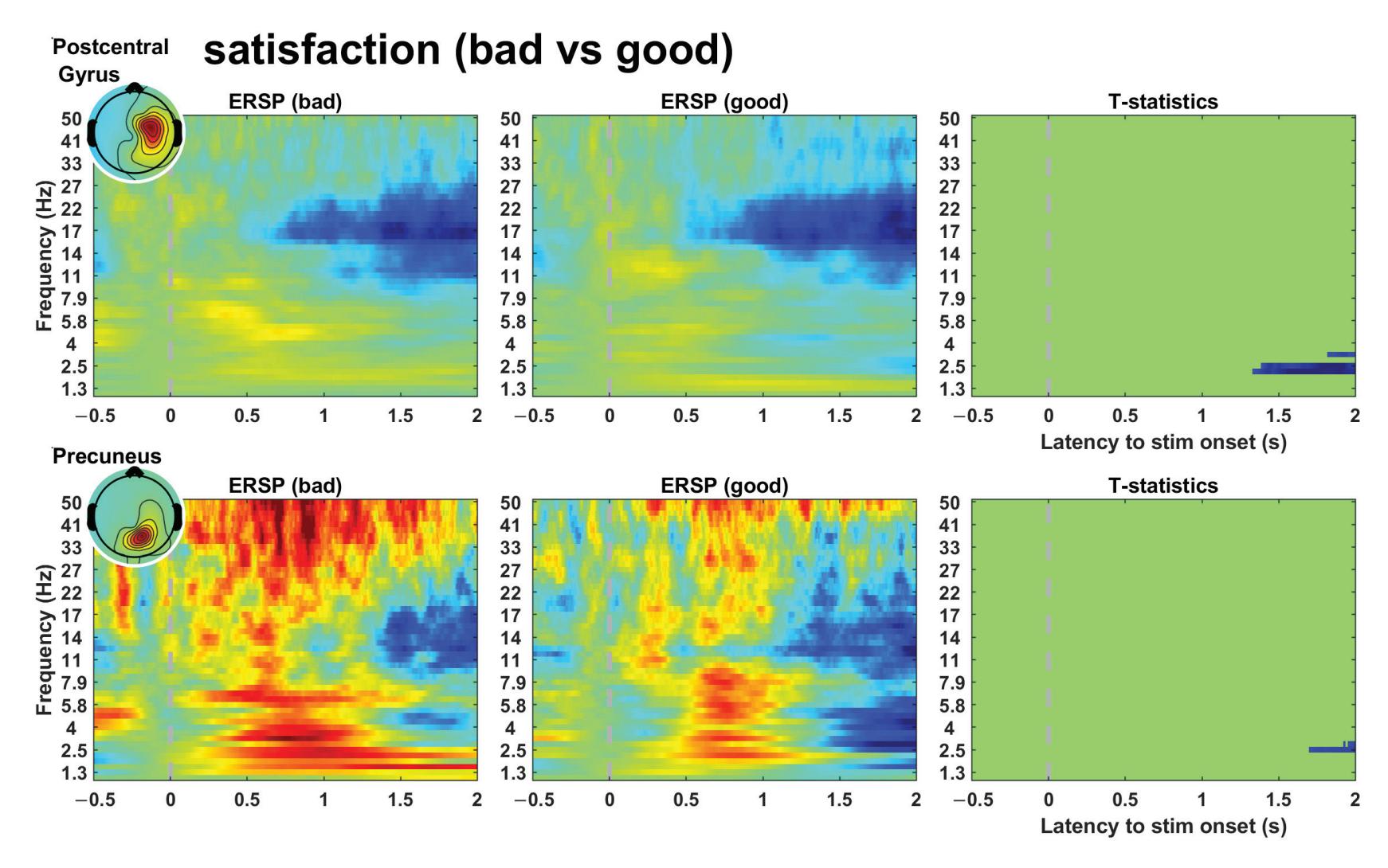
**Figure 3.** Event-related spectral perturbation of clusters including a significant area in the comparison of satisfaction. The dotted line represents the onset of the "Go" cue. In each figure set, the third column represents t-statistics and the significant area. This plot indicates that satisfaction is determined dominantly in the final phase of control.
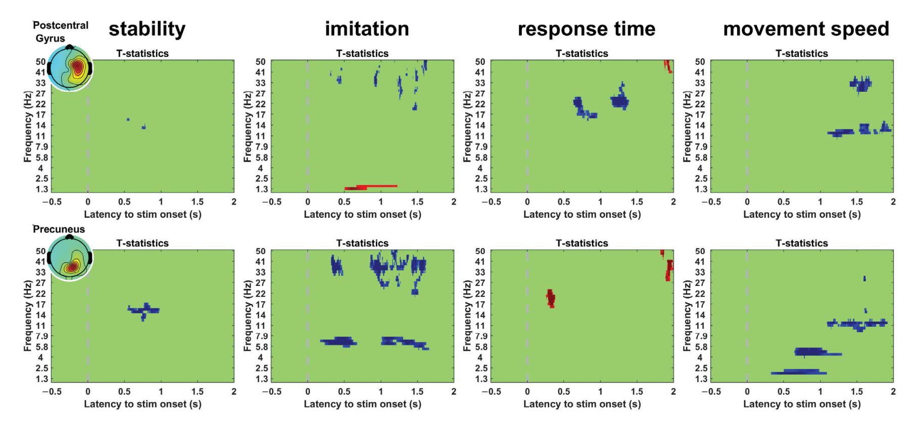
**Figure 4.** Significant areas in the comparisons; stability (unstable vs. stable), imitation (bad vs. good), response time (delayed vs. no delay), and movement speed (extremely slow vs. extremely fast). The dotted line represents the onset of the "Go" cue. The blue areas represent negative t-statistics, and the red areas represent positive t-statistics.
136
*Sensors* **2023**, *23*, 277
**Table 2.** T-statistics of significant areas.
| Indicator | Cluster | Mean | Min (or Max) |
|---------------|------------------------|-------|--------------|
| Stability | Precuneus | -3.79 | -5.83 |
| Imitation | Postcentral (increase) | 3.26 | 3.89 |
| Imitation | Postcentral (decrease) | -3.49 | -6.15 |
| Imitation | Precuneus | -3.01 | -7.85 |
| Response time | Postcentral (increase) | 3.45 | 4.28 |
| Response time | Postcentral (decrease) | -3.8 | -6.81 |
| Response time | Precuneus | 3.99 | 6.66 |
| Speed | Postcentral | -3.63 | -5.73 |
| Speed | Precuneus | -3.79 | -5.42 |
| Satisfaction | Postcentral | -3.69 | -4.30 |
| Satisfaction | Precuneus | -3.22 | -3.49 |
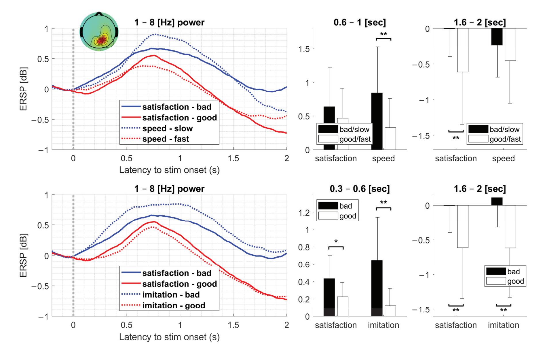
**Figure 5.** Power (1–8 Hz) of the clusters related to the precuneus. We extracted powers within the range of 1–8 Hz shown as a significant area in ERSP. The comparison of the movement speed exhibited a power difference within the range of 0.6–1 s, although the power difference in satisfaction was not significant. Although the power difference within the range of 1.6–2 s was significant in the comparison of satisfaction and imitation, the difference in the movement speed was not. Within the range of 0.3–0.6 s, satisfaction exhibited a moderate difference, and imitation exhibited a more significant difference. All tests were performed by *t*-test (\*: *p* < 0.05; \*\*: *p* < 0.01).
137
*Sensors* **2023**, *23*, 277
#### 4. Discussion
By using the participants' responses to the questionnaire, we investigated the reflection of brain activity on user satisfaction alongside performance indicators of EMG-based robot control. We found that two clusters primarily linked satisfaction and the indicators, as shown in Figure 2. Brain activity exhibited significant differences in satisfaction at a later stage but not immediately after feeding an input, as shown in Figure 3. The indicators exhibited their independent significant patterns in ERSPs, as shown in Figure 4.
User satisfaction exhibited significant differences primarily at the end of the epoch. This could imply that the level of satisfaction was primarily determined by the latest information, regardless of the robotic performance immediately after an input command. This might be a specific characteristic of satisfaction in the brain determined by the latest information. This has rarely been discovered in a study on user satisfaction in human–robot interaction [23]. However, a previous study on user satisfaction with a haptic interface reported that EEG power in the early period exhibited a significant correlation with user satisfaction [24]. The reported results revealed that each participant exhibited different frequency bands (alpha, delta, and high gamma), primarily contributing to satisfaction. We conjecture that the experiment in the previous study asked participants only about satisfaction, which would have different meanings depending on the individual. In our questionnaire, we suggested multiple indicators, which might have enabled the participants to limit their interpretation of satisfaction. In addition, different interface environments could define different satisfaction levels. In a dial interface, gamma EEG over the frontal area in the early period exhibited a significant contribution to satisfaction [25]. Additionally, some studies have reported that different paradigms exhibited different preferences in a brain–computer interface using motor imagery [26].
Among the four indicators, stability exhibited a significant difference in a portion of the epoch. However, the other indicators exhibited significant differences in most of the epochs. Several independent activations appeared to be involved in significant areas in response time and movement speed. The cluster related to the precuneus exhibited an earlier and more significant difference than the other clusters, indicating that movement speed and delay might be processed as information about a fundamental concept through the precuneus within the brain. As visual information is processed in two pathways, this might reflect the process on the dorsal pathway. Humans can intuitively recognize delay and speed immediately as they observe a robotic movement. However, considerable time is required to recognize stability, indicating that stability is represented as integrated information in the brain. Another high-level concept is the sense of agency, which refers to the feeling of control [27] and is dependent on delay and speed. Delay has been used to reduce the sense of agency [28]. A previous study reported that the speed of controlled objects is also related to the sense of agency [29]. This supports the idea that delay and speed are the fundamental factors affecting subjective feelings. Although delay appears to be a low-level concept, its effect is complex. Participants sometimes fail to perceive the correct delay [5]. Moreover, the awareness between certainty and uncertainty with respect to the delayed response of a robotic hand can induce a significant difference in the theta band of the parietal lobe [30]. Additionally, although unlike delay, imitation is not a simple concept, significant differences were observed immediately after the onset. This might be caused by differences in the gamma band related to sensory awareness [31,32], which may have influenced subjective feelings. The significant gamma powers in the other interval might be related to emotional processing [33].
In all the indicators, including satisfaction, the pattern of significant regions in one of the clusters resembled the pattern of the other cluster in the time–frequency plot, implying that the two clusters may be functionally connected and reflect information flow between them. Moreover, the gamma power in imitation, gamma power at the end of the epoch in the response time, and alpha power in the movement speed exhibited a larger difference area in the precuneus-related clusters than in the postcentral-gyrus-related cluster. Furthermore, user satisfaction exhibited a longer and larger significant area in the postcentral gyrus than
138
*Sensors* **2023**, *23*, 277
in the precuneus. Considering the visual information pathway through the parietal area, satisfaction is primarily determined by other integrated information, unlike information through the precuneus at that time.
We used a k-means algorithm for clustering based on the dipole locations. However, several other methods could be used for clustering, such as hierarchical clustering or a sequential algorithm of partitional clustering. In this case, other features could be included for optimized clustering besides dipole location. These features should be investigated in future studies so that optimized components related to the task or stimulus can be extracted.
As the ERSPs in the low-frequency band were related to satisfaction, we compared them with imitation and movement speed, which exhibited significant differences. The speed indicator showed that the difference between powers within the range of 0.6–1 s was significant, whereas satisfaction exhibited a significant difference within the range of 1.6–2 s. This may imply that speed is not a primary contributor to satisfaction. For imitation, powers within the ranges of 0.3–0.6 s and 1.6–2 s exhibited significant differences. Satisfaction also exhibited significant differences in both intervals, but the difference in the early period was moderate. As imitation covered significant intervals in satisfaction, it was the most important contributing factor among the four indicators. We presented the indicators as evaluation indicators regardless of the participant's satisfaction. Our results reveal that objective performance evaluation, regardless of subjective satisfaction, can fully reflect satisfaction. As no optimal control configurations exist, the robot system should evaluate the user's satisfaction without measuring satisfaction. In other words, satisfaction should be estimated using information that the robot system can exploit. Our results prove the feasibility of this method with brain-related signals. However, the information that contributed to satisfaction was not a simple parameter such as delay or movement speed. The fundamental unit satisfaction processing in the brain might be neither of these factors. Although we have yet to elucidate the representation of imitation in the brain, we discovered integrated information related to a robot's objective movement, causing satisfaction to be processed in the brain. In future studies, integrated information, which might consist of basic parameters such as delay and movement speed, should be investigated to ensure the decomposition of integrated information and determine more direct contributors to satisfaction. Then, the information could be exploited to determine individualized optimal parameters and used to generalize individualized preferred robot configurations.
**Author Contributions:** Conceptualization, H.K., N.Y. and Y.K. (Yasuharu Koike); Methodology, H.K., M.M. and Y.K. (Yasuharu Koike); Software, H.K., M.M., Y.K. (Yeongdae Kim) and S.S.; Validation, H.K., M.M., N.Y. and Y.K. (Yasuharu Koike); Formal analysis, H.K. and M.M.; Investigation, H.K. and M.M.; Data curation, H.K., Y.K. (Yeongdae Kim) and S.S.; Writing—original draft, H.K., M.M., N.Y. and Y.K. (Yasuharu Koike); Writing—review & editing, H.K., M.M., N.Y. and Y.K. (Yasuharu Koike); Supervision, N.Y. and Y.K. (Yasuharu Koike); Project administration, Y.K. (Yasuharu Koike); Funding acquisition, Y.K. (Yasuharu Koike). All authors have read and agreed to the published version of the manuscript.
**Funding:** This work was supported by JSPS under KAKENHI grant number 19H05728 and the Tateisi Science and Technology Foundation (grant number 2188001).
**Institutional Review Board Statement:** The study was conducted in accordance with the Declaration of Helsinki, and approved by the Institutional Review Board (or Ethics Committee) of Tokyo Institute of Technology (protocol code 2019002 and date of approval 1 April 2019).
**Informed Consent Statement:** Informed consent was obtained from all subjects involved in the study.
**Data Availability Statement:** The data presented in this study are available on request from the corresponding author.
**Conflicts of Interest:** The authors declare no conflict of interest.
139
*Sensors* **2023**, *23*, 277
#### References
- 1. Connan, M.; Ruiz Ramírez, E.; Vodermayer, B.; Castellini, C. Assessment of a wearable force- and electromyography device and comparison of the related signals for myocontrol. *Front. Neurorobotics* **2016**, *10*, 17. [CrossRef] [PubMed]
- 2. Barszap, A.G.; Skavhaug, I.-M.; Joshi, S.S. Effects of muscle fatigue on the usability of a myoelectric human-computer interface. *Hum. Mov. Sci.* **2016**, *49*, 225–238. [CrossRef]
- 3. Belyea, A.; Englehart, K.; Scheme, E. FMG Versus EMG: A Comparison of Usability for Real-Time Pattern Recognition Based Control. *IEEE Trans. Biomed. Eng.* **2019**, *66*, 3098–3104. [CrossRef] [PubMed]
- 4. Poritz, J.M.P.; Taylor, H.B.; Francisco, G.; Chang, S.-H. User satisfaction with lower limb wearable robotic exoskeletons. *Disabil. Rehabil. Assist. Technol.* **2020**, *15*, 322–327. [CrossRef]
- 5. Kim, H.; Yoshimura, N.; Koike, Y. Investigation of Delayed Response during Real-Time Cursor Control Using Electroencephalography. *J. Healthc. Eng.* **2020**, *2020*, 1418437. [CrossRef] [PubMed]
- 6. Dennis, T.A.; Solomon, B. Frontal EEG and emotion regulation: Electrocortical activity in response to emotional film clips is associated with reduced mood induction and attention interference effects. *Biol. Psychol.* **2010**, *85*, 456–464. [CrossRef] [PubMed]
- 7. Lee, M.; Shin, G.-H.; Lee, S.-W. Frontal EEG asymmetry of emotion for the same auditory stimulus. *IEEE Access* **2020**, *8*, 107200–107213. [CrossRef]
- 8. Plourde-Kelly, A.D.; Saroka, K.S.; Dotta, B.T. The impact of emotionally valenced music on emotional state and EEG profile: Convergence of self-report and quantitative data. *Neurosci. Lett.* **2021**, *758*, 136009. [CrossRef]
- 9. Wang, J.; Wang, M. Review of the emotional feature extraction and classification using EEG signals. *Cogn. Robot.* **2021**, *1*, 29–40. [CrossRef]
- 10. Rabcan, J.; Levashenko, V.; Zaitseva, E.; Kvassay, M. Review of methods for EEG signal classification and development of new fuzzy classification-based approach. *IEEE Access* **2020**, *8*, 189720–189734. [CrossRef]
- 11. Callejas-Cuervo, M.; González-Cely, A.X.; Bastos-Filho, T. Control systems and electronic instrumentation applied to autonomy in wheelchair mobility: The state of the art. *Sensors* **2020**, *20*, 6326. [CrossRef]
- 12. Koike, Y.; Kim, Y.; Stapornchaisit, S.; Qin, Z.; Kawase, T.; Yoshimura, N. Development of Multi-sensor Array Electrodes for Measurement of Deeper Muscle Activation. *Sens. Mater.* **2020**, *32*, 959. [CrossRef]
- 13. Cichocki, A.; Phan, A.-H. Fast local algorithms for large scale nonnegative matrix and tensor factorizations. *IEICE Trans. Fundam. Electronics. Commun. Comput. Sci.* **2009**, *E92-A*, 708–721. [CrossRef]
- 14. Kawase, T.; Sakurada, T.; Koike, Y.; Kansaku, K. A hybrid BMI-based exoskeleton for paresis: EMG control for assisting arm movements. *J. Neural Eng.* **2017**, *14*, 016015. [CrossRef]
- 15. Delorme, A.; Makeig, S. EEGLAB: An open source toolbox for analysis of single-trial EEG dynamics including independent component analysis. *J. Neurosci. Methods* **2004**, *134*, 9–21. [CrossRef]
- 16. Bigdely-Shamlo, N.; Mullen, T.; Kothe, C.; Su, K.-M.; Robbins, K.A. The PREP pipeline: Standardized preprocessing for large-scale EEG analysis. *Front. Neuroinf.* **2015**, *9*, 16. [CrossRef]
- 17. Mullen, T.R.; Kothe, C.A.E.; Chi, Y.M.; Ojeda, A.; Kerth, T.; Makeig, S.; Jung, T.-P.; Cauwenberghs, G. Real-Time Neuroimaging and Cognitive Monitoring Using Wearable Dry EEG. *IEEE Trans. Biomed. Eng.* **2015**, *62*, 2553–2567. [CrossRef]
- 18. Blum, S.; Jacobsen, N.S.J.; Bleichner, M.G.; Debener, S. A riemannian modification of artifact subspace reconstruction for EEG artifact handling. *Front. Hum. Neurosci.* **2019**, *13*, 141. [CrossRef]
- 19. Piazza, C.; Miyakoshi, M.; Akalin-Acar, Z.; Cantiani, C.; Reni, G.; Bianchi, A.M.; Makeig, S. An Automated Function for Identifying EEG Independent Components Representing Bilateral Source Activity. In Proceedings of the XIV Mediterranean Conference on Medical and Biological Engineering and Computing, Paphos, Cyprus, 31 March–2 April 2016; Kyriacou, E., Christofides, S., Pattichis, C.S., Eds.; IFMBE Proceedings. Springer International Publishing: Cham, Switzerland, 2016; Volume 57, pp. 105–109.
- 20. Pion-Tonachini, L.; Kreutz-Delgado, K.; Makeig, S. ICLabel: An automated electroencephalographic independent component classifier, dataset, and website. *Neuroimage* **2019**, *198*, 181–197. [CrossRef]
- 21. Rousseeuw, P.J. Silhouettes: A graphical aid to the interpretation and validation of cluster analysis. *J. Comput. Appl. Math.* **1987**, *20*, 53–65. [CrossRef]
- 22. Groppe, D.M.; Urbach, T.P.; Kutas, M. Mass univariate analysis of event-related brain potentials/fields I: A critical tutorial review. *Psychophysiology* **2011**, *48*, 1711–1725. [CrossRef] [PubMed]
- 23. Esfahani, E.T.; Sundararajan, V. Using brain–computer interfaces to detect human satisfaction in human–robot interaction. *Int. J. Human. Robot.* **2011**, *8*, 87–101. [CrossRef]
- 24. Park, W.; Ki, D.; Kim, D.H.; Kwon, G.H.; Kim, S.P.; Kim, L. EEG correlates of user satisfaction of haptic sensation. In Proceedings of the 2015 IEEE International Conference on Consumer Electronics (ICCE), Las Vegas, NV, USA, 9–12 January 2015; pp. 569–570.
- 25. Park, W.; Kim, D.-H.; Kim, S.-P.; Lee, J.-H.; Kim, L. Gamma EEG correlates of haptic preferences for a dial interface. *IEEE Access* **2018**, *6*, 22324–22331. [CrossRef]
- 26. Song, M.; Kim, J. A Paradigm to Enhance Motor Imagery Using Rubber Hand Illusion Induced by Visuo-Tactile Stimulus. *IEEE Trans. Neural Syst. Rehabil. Eng.* **2019**, *27*, 477–486. [CrossRef]
- 27. Haggard, P. Sense of agency in the human brain. *Nat. Rev. Neurosci.* **2017**, *18*, 196–207. [CrossRef] [PubMed]
- 28. Wen, W. Does delay in feedback diminish sense of agency? A review. *Conscious Cogn.* **2019**, *73*, 102759. [CrossRef]
- 29. Kawabe, T. Inferring sense of agency from the quantitative aspect of action outcome. *Conscious Cogn.* **2013**, *22*, 407–412. [CrossRef]
140
*Sensors* **2023**, *23*, 277
- 30. Kim, H.; Kim, Y.; Miyakoshi, M.; Stapornchaisit, S.; Yoshimura, N.; Koike, Y. Brain Activity Reflects Subjective Response to Delayed Input When Using an Electromyography-Controlled Robot. *Front. Syst. Neurosci.* **2021**, *15*, 767477. [CrossRef]
- 31. Engel, A.K.; Singer, W. Temporal binding and the neural correlates of sensory awareness. *Trends Cogn. Sci. (Regul. Ed.)* **2001**, *5*, 16–25. [CrossRef]
- 32. Rieder, M.K.; Rahm, B.; Williams, J.D.; Kaiser, J. Human γ-band activity and behavior. *Int. J. Psychophysiol.* **2011**, *79*, 39–48. [CrossRef]
- 33. Matsumoto, A.; Ichikawa, Y.; Kanayama, N.; Ohira, H.; Iidaka, T. Gamma band activity and its synchronization reflect the dysfunctional emotional processing in alexithymic persons. *Psychophysiology* **2006**, *43*, 533–540. [CrossRef] [PubMed]
**Disclaimer/Publisher's Note:** The statements, opinions and data contained in all publications are solely those of the individual author(s) and contributor(s) and not of MDPI and/or the editor(s). MDPI and/or the editor(s) disclaim responsibility for any injury to people or property resulting from any ideas, methods, instructions or products referred to in the content.
141


*Article*
### Comprehensive Analysis of Feature Extraction Methods for Emotion Recognition from Multichannel EEG Recordings
**Rajamanickam Yuvara 1,\*, Prasanth Thagavel 2, John Thomas 3, Jack Fogarty 1 and Farhan Ali 1**
- 1 National Institute of Education, Nanyang Technological University, Singapore 637616, Singapore
- 2 Interdisciplinary Graduate School, Nanyang Technological University, Singapore 639798, Singapore
- 3 Montreal Neurological Institute, McGill University, Montreal, QC H3A 2B4, Canada
- **\*** Correspondence: yuvaraj.rajamanickam@nie.edu.sg; Tel.: +65-94817650
**Abstract:** Advances in signal processing and machine learning have expedited electroencephalogram (EEG)-based emotion recognition research, and numerous EEG signal features have been investigated to detect or characterize human emotions. However, most studies in this area have used relatively small monocentric data and focused on a limited range of EEG features, making it difficult to compare the utility of different sets of EEG features for emotion recognition. This study addressed that by comparing the classification accuracy (performance) of a comprehensive range of EEG feature sets for identifying emotional states, in terms of valence and arousal. The classification accuracy of five EEG feature sets were investigated, including statistical features, fractal dimension (FD), Hjorth parameters, higher order spectra (HOS), and those derived using wavelet analysis. Performance was evaluated using two classifier methods, support vector machine (SVM) and classification and regression tree (CART), across five independent and publicly available datasets linking EEG to emotional states: MAHNOB-HCI, DEAP, SEED, AMIGOS, and DREAMER. The FD-CART featureclassification method attained the best mean classification accuracy for valence (85.06%) and arousal (84.55%) across the five datasets. The stability of these findings across the five different datasets also indicate that FD features derived from EEG data are reliable for emotion recognition. The results may lead to the possible development of an online feature extraction framework, thereby enabling the development of an EEG-based emotion recognition system in real time.
**Keywords:** EEG; emotion recognition; EEG feature extraction; valence; arousal; pattern recognition
**Citation:** Yuvaraj, R.; Thagavel, P.; Thomas, J.; Fogarty, J.; Ali, F. Comprehensive Analysis of Feature Extraction Methods for Emotion Recognition from Multichannel EEG Recordings. *Sensors* **2023**, *23*, 915. https://doi.org/10.3390/s23020915
Academic Editors: Yifan Zhao, Fei He and Yuzhu Guo
Received: 22 December 2022 Revised: 7 January 2023 Accepted: 9 January 2023 Published: 12 January 2023

**Copyright:** © 2023 by the authors. Licensee MDPI, Basel, Switzerland. This article is an open access article distributed under the terms and conditions of the Creative Commons Attribution (CC BY) license (https:// creativecommons.org/licenses/by/ 4.0/).
#### 1. Introduction
Emotions have a complex and fundamental role in cognition and behavior, influencing how we interact with and interpret our daily life experiences. Technology that can help recognize and measure emotions is highly desirable, as this can facilitate research and development in areas such as healthcare, education, psychology, robotics, marketing, and entertainment. Emotion recognition technology can also offer individuals (or clinicians) tools to aid emotion regulation and intervention. However, despite years of interest in psychology and affective computing, the development of reliable and generalizable emotion detection techniques is still a challenge. To that end, this study provides a comprehensive analysis of electroencephalogram (EEG) measures of emotional states, categorized in terms of valence (positive vs. negative) and arousal (high vs. low).
Numerous experiments on emotion recognition have been undertaken in recent years utilizing both physiological signals (e.g., electrocardiogram (ECG), galvanic skin resistance (GSR), electromyogram (EMG), respiration rate (RR), electrodermal activity (EDA) and EEG signals) [1,2] and behavioral data (e.g., facial expression images, body gestures, speech and voice signals) [3,4]. Behavioral data can provide useful measures of emotion-related processes; however, they can also be easily biased due to their subjective and controllable nature. In comparison, physiological signals are relatively automatic and uncontrolled
*Sensors* **2023**, *23*, 915. https://doi.org/10.3390/s23020915 https://www.mdpi.com/journal/sensors
142

*Article*
# Comprehensive Analysis of Feature Extraction Methods for Emotion Recognition from Multichannel EEG Recordings
**Rajamanickam Yuvara 1,\*, Prasanth Thagavel 2, John Thomas 3, Jack Fogarty 1 and Farhan Ali 1**
- 1 National Institute of Education, Nanyang Technological University, Singapore 637616, Singapore
- 2 Interdisciplinary Graduate School, Nanyang Technological University, Singapore 639798, Singapore
- 3 Montreal Neurological Institute, McGill University, Montreal, QC H3A 2B4, Canada
- **\*** Correspondence: yuvaraj.rajamanickam@nie.edu.sg; Tel.: +65-94817650
**Abstract:** Advances in signal processing and machine learning have expedited electroencephalogram (EEG)-based emotion recognition research, and numerous EEG signal features have been investigated to detect or characterize human emotions. However, most studies in this area have used relatively small monocentric data and focused on a limited range of EEG features, making it difficult to compare the utility of different sets of EEG features for emotion recognition. This study addressed that by comparing the classification accuracy (performance) of a comprehensive range of EEG feature sets for identifying emotional states, in terms of valence and arousal. The classification accuracy of five EEG feature sets were investigated, including statistical features, fractal dimension (FD), Hjorth parameters, higher order spectra (HOS), and those derived using wavelet analysis. Performance was evaluated using two classifier methods, support vector machine (SVM) and classification and regression tree (CART), across five independent and publicly available datasets linking EEG to emotional states: MAHNOB-HCI, DEAP, SEED, AMIGOS, and DREAMER. The FD-CART featureclassification method attained the best mean classification accuracy for valence (85.06%) and arousal (84.55%) across the five datasets. The stability of these findings across the five different datasets also indicate that FD features derived from EEG data are reliable for emotion recognition. The results may lead to the possible development of an online feature extraction framework, thereby enabling the development of an EEG-based emotion recognition system in real time.
**Keywords:** EEG; emotion recognition; EEG feature extraction; valence; arousal; pattern recognition

**Citation:** Yuvaraj, R.; Thagavel, P.; Thomas, J.; Fogarty, J.; Ali, F. Comprehensive Analysis of Feature Extraction Methods for Emotion Recognition from Multichannel EEG Recordings. *Sensors* **2023**, *23*, 915. https://doi.org/10.3390/s23020915
Academic Editors: Yifan Zhao, Fei He and Yuzhu Guo
Received: 22 December 2022 Revised: 7 January 2023 Accepted: 9 January 2023 Published: 12 January 2023

**Copyright:** © 2023 by the authors. Licensee MDPI, Basel, Switzerland. This article is an open access article distributed under the terms and conditions of the Creative Commons Attribution (CC BY) license (https:// creativecommons.org/licenses/by/ 4.0/).
## 1. Introduction
Emotions have a complex and fundamental role in cognition and behavior, influencing how we interact with and interpret our daily life experiences. Technology that can help recognize and measure emotions is highly desirable, as this can facilitate research and development in areas such as healthcare, education, psychology, robotics, marketing, and entertainment. Emotion recognition technology can also offer individuals (or clinicians) tools to aid emotion regulation and intervention. However, despite years of interest in psychology and affective computing, the development of reliable and generalizable emotion detection techniques is still a challenge. To that end, this study provides a comprehensive analysis of electroencephalogram (EEG) measures of emotional states, categorized in terms of valence (positive vs. negative) and arousal (high vs. low).
Numerous experiments on emotion recognition have been undertaken in recent years utilizing both physiological signals (e.g., electrocardiogram (ECG), galvanic skin resistance (GSR), electromyogram (EMG), respiration rate (RR), electrodermal activity (EDA) and EEG signals) [1,2] and behavioral data (e.g., facial expression images, body gestures, speech and voice signals) [3,4]. Behavioral data can provide useful measures of emotion-related processes; however, they can also be easily biased due to their subjective and controllable nature. In comparison, physiological signals are relatively automatic and uncontrolled *Sensors* **2023**, *23*, 915. https://doi.org/10.3390/s23020915 https://www.mdpi.com/journal/sensors
142
*Sensors* **2023**, *23*, 915
and, therefore, may capture processes that can distinguish an individual's true (unbiased) emotional states more objectively. Thus, relative to behavioral data, physiological signalbased emotion recognition has fundamental advantages in terms of reliability and validity.
A range of physiological signals have been explored for emotion recognition [1,5]. However, relative to other modalities, techniques based on EEG data have received remarkable attention due to the direct link between EEG and the neurophysiological activity of the central nervous system, as well as its high time resolution and reliability. Furthermore, due to the rapid advancement of sensor technology EEG data collection is becoming more practical. Considering the popularity of EEG as a measure of emotion, and its increasing accessibility for researchers and consumers, this current study is focused on EEG-based emotion recognition. Despite the large number of studies conducted on EEG-based emotion recognition, there are unsolved issues and questions. For example, the number of emotion classes recognized, the number of electrodes used, the accuracy of emotion recognition, and the generalization of the emotion recognition task.
To detect emotions using EEG, researchers traditionally extract a range of signal properties referred to as 'features', which are then analyzed relative to emotions (or emotion processing), to explore their utility for detecting or classifying experienced emotions. The accuracy of emotion recognition will be largely influenced by the quality of feature extraction and their functional relevance (or significance) to emotions. Until now, few EEG studies have been performed to compare the importance of different EEG features that are often used for emotion recognition. Schaaff and Schultz [6] compared classification accuracy of pleasant, neutral, and unpleasant emotional state among two different sets of features measured in the time domain (e.g., statistical), and frequency domain (e.g., Fast Fourier Transform) . Petrantonakis et al. [7] computed the higher order crossing (HOC) features of EEG signals and evaluated their performance in classifying emotional states (such as happiness, surprise, anger, fear, disgust, and sadness) among statistical and wavelet-based features. Frantzidis et al. [8] suggested using the Event Related Potential (ERP) amplitude, ERP latency and Event Related Oscillation (ERO) amplitude as features for emotional state classification . In [9], the authors performed time–frequency analysis to assess the event related synchronization (ERS)/desynchronization (ERD) characteristics of EEG data and compared liking and disliking emotional states across various time–frequency ERS/ERD features. Jenke et al. [10] explored multiple features such as band power, HOC, fractal dimension (FD), discrete wavelet transform (DWT), Hilbert–Huang spectrum, differential asymmetry, and rational asymmetry. They compared the classification of happy, curious, angry, sad, and quiet emotional state among different feature vectors. Liu and Sourina [11] computed FD features and compared the performance with statistical features for valence recognition. Yuvaraj et al. [12] employed bispectrum features for basic emotional state classification and compared the classification performance with power spectrum, wavelet packet and nonlinear features. Recently, Nawaz et al. [13] proposed an emotion recognition framework based on the statistical features and evaluated the classification accuracy in comparison to power, wavelet, and entropy features. Together, these studies indicate the potential to detect or characterize basic emotional state using various EEG feature sets. However, it is difficult to compare the performance of feature sets across the different studies as most analyses were performed using only on handful of features, thus failing to provide insight into their relative utility for developing automated (i.e., online) systems that can understand or classify human emotions in applied settings. Furthermore, many studies were evaluated only on a monocentric data (i.e., single, or smaller dataset), typically collected from on a smaller cohort.
The present study aims to provide the most comprehensive analysis of different EEG feature sets for emotion recognition to date to determine which features are best for distinguishing emotional states, categorized in terms of valence and arousal. To achieve this, a wide range of features are analyzed across five public datasets to identify the most significant and generalizable EEG features distinguishing high/low emotional valence and arousal states; the five public datasets used in this study are, DEAP [14], DREAMER [15], 143
*Sensors* **2023**, *23*, 915
MAHNOB-HCI [16], AMIGOS [17] and SEED [18]. The feature sets that are explored include statistical, fractal dimension (FD), Hjorth parameters, higher order spectra (HOS), and wavelet transform. Like in most machine learning studies (e.g., [7,12,13]), classification accuracy serves as the main performance metric in this investigation; however, given that machine learning accuracy can vary across classification techniques [7,12,13], we also test the performance of two common classifiers, specifically, support vector machine (SVM) and classification and regression tree (CART). In this way, we aim to recommend the most useful and generalizable EEG feature-classification technique for detecting emotional states and to guide the future development of emotion recognition systems.
The key contributions of the current study are the following: We (i) evaluated the performance using five independent and public EEG emotion datasets and (ii) identified the optimal feature set for reliable EEG-based emotional state recognition. To our knowledge, this study could be one of the first to utilize five independent public datasets to identify the optimal EEG feature set that can discriminate emotions. The rest of the work is arranged as follows. The scalp EEG datasets and the details of the method are explained in Section 2. Various experimental results and discussions are described in Section 3. Last, Section 4 covers the conclusions.
## 2. Materials and Methods
Figure 1 shows the methodological framework of the EEG and machine learning techniques used in the present study. For each EEG dataset (described in Section 2.1), the raw EEG data was subjected to (1) preprocessing, (2) feature extraction, and (3) emotional state classification based on ground-truth self-report data reflecting emotional valence and/or arousal.
**Figure 1.** An overview of the proposed machine learning framework for emotion recognition based on EEG signals.
### 2.1. Emotion-Related EEG Datasets
This study utilizes emotion-related EEG signals from the five most popularly used public datasets, namely MAHNOB-HCI, DEAP (Dataset for Emotion Analysis using Physiological signals), SEED (SJUT emotion EEG Dataset), AMIGOS (A dataset for Mood, personality, and affect research on individuals and GrOupS), and DREAMER. Table 1 summarizes the core details of these datasets that are relevant to the present research, including sample characteristics and EEG parameters. Datasets include EEG recordings from 15–40 (*M* = 27.4, *SD* = 9.4) young adult participants (55% male overall), recorded using different EEG systems with 14–62 scalp channels. The specifics of each dataset are described in detail in the subsequent paragraphs.
The MAHNOB-HCI was pioneered by Soleymani and fellows [16], which comprises of 32-channel EEG recordings and other peripheral nervous system (PNS) signals. The signals were obtained from 27 participants as they watched 20 video clips, which lasted from 34.9 s 144
*Sensors* **2023**, *23*, 915
to 117 s. Participants rated their levels in valence, arousal, dominance, and predictability, after they watched each clip. The DEAP emotion dataset is a multimodal dataset created by [14], which comprises EEG signals from 32-channels and other PNS signals. These signals were collected from 32 healthy subjects when they were watching 40 music video clips (i.e., 40 trials in total), each video clip lasting a minute. After each video/trial, the participants were asked to rate their arousal, valence, dominance, like/dislike, and familiarity level using self-assessment report. The data of each video consists of 60-s EEG recordings and a 3 s baseline data. The EEG were collected with the sampling frequency *(Fs)* of 512 Hz. The SEED dataset [18] comprises EEG and eye movement signals from 15 participants exhibiting three different emotions namely positive, negative, and neutral emotional state. Each participant had three experiment sessions on different days. In each session, there were fifteen four-minute videos to evoke the required emotions. Therefore, for the three sessions, there are 45 trials in the database. The same fifteen videos were used in all three experiment sessions. The EEG signals were collected from 62 channels with *Fs* = 1000 Hz and down sampled to 200 Hz. After each session, the participants were asked to label the video according to the contents: −1 for negative, 0 for neutral, and 1 for positive. In this study, we employed only recordings with positive and negative labels from participants to assess our results with additional emotion datasets that apply binary classifiers.
**Table 1.** Information about the datasets used in this study.
| Public
Dataset
Name | Pub.
Year | Sample
Size
(N) | Gender Ratio
(Mean
Age ± SD) | Total
Trials
or
Videos | Trial/
Video
Dura. | Rec.
Ses. | # EEG Channels
/Device
/Fs | Emotional
States | Rating
Scale
Ranges
(Thres.) |
|---------------------------|--------------|-----------------------|------------------------------------|---------------------------------|--------------------------|--------------|-------------------------------------|------------------------|---------------------------------------|
| MAHNOB
-HCI | 2011 | 27 | 11M /16F
(NS
± NS) | 20 | 34.92
to
117 s | 1 | 32/
BioSemi Active II
/256 Hz | Valence &
Arousal | 1–9
(4.5) |
| DEAP | 2012 | 32 | 16M/16F
(26.9
± NS) | 40 | 60 s | 1 | 32/
BioSemi Active II
/512 Hz | Valence &
Arousal | 1–9
(4.5) |
| SEED | 2015 | 15 | 7M/8F
(23.27
± 2.37) | 10 | ∼240 s | 3 | 62/
ESI Neuro Scan
/1000 Hz | Positive &
Negative | −1, 0, & 1
(NA) |
| AMIGOS | 2018 | 40 | 27M/13F
(28.3
± NS) | 16 | <250 s | 2 | 14/
Emotive EPOC
/128 Hz | Valence &
Arousal | 1–9
(4.5) |
| DREAMER | 2018 | 23 | 14M/9F
(26.6
± 2.7) | 18 | 65–393 s | 1 | 14/
Emotiv EPO
/128 Hz | Valence &
Arousal | 1–5
(2.5) |
All the EEGs are recorded using the international 10–20 positioning system. Fs = sampling frequency in Hz, M = Male, F = Female, SD = standard deviation, s = seconds, NS = not specified, NA = not applicable, Pub. publication, dura.—duration, Rec.—recording, ses.—sessions, thres.—threshold.
The AMIGOS dataset [17] includes 14 channels of EEG data, 2 channels of ECG data, galvanic skin response, and frontal video. The dataset was prepared from the recordings of 40 participants when they viewed 16 film clips, which lasted no longer than 250 s. After seeing each movie clip, participants self-assessed their levels of arousal, valence, dominance, liking, familiarity, and seven fundamental emotions (happiness, disgust, surprise, fear, anger, sorrow and neutral). As stated in [19], seven participants (participant ID: 9, 12, 21, 22, 23, 24, 29, and 33) physiological signals had missing data, therefore we excluded them in our study. Some participants (participant ID: 5, 11, 28, and 30) did not have either valence or arousal affective state values, so we excluded their data as well. The DREAMER dataset was developed by [15] and comprised of EEG signals from 14 channels and 2-channel ECG signals. These signals were collected from 23 healthy participants (aged between 22 and 33 years) as they watched 18 video clips with lengths between 65 and 393 s. After every video clip, the participants assessed their degrees of arousal, valence, and dominance using
145
*Sensors* **2023**, *23*, 915
self-assessment manikin (SAM). In addition, 60-second baseline signals were recorded before each clip. EEG signals were captured with an Emotive EPOC wireless neuro headset with *Fs* of 128 Hz.
In this study, only the raw EEG and self-report data reflecting emotional valence and arousal were extracted for analyses. Furthermore, to be consistent across datasets, only data from the first session was used from sets including multiple sessions (i.e., AMIGOS and SEED). Across all datasets, and in this study, emotional valence and arousal (Figure 2) were analyzed as two orthogonal dimensions [19–21], consistent with popular circumplex models of emotion (e.g., [22]). The self-report scales used to rate valence and arousal differed across datasets; for DEAP, MANHOB-HCI, and AMIGOS each dimension was rated on a scale of 1 to 9, whereas for DREAMER, they were rated from 1 to 5, with lower numbers reflecting more negative or lower valence and arousal, respectively. To test and validate EEG classification of emotion, EEG data were first categorized as either low or high valence and arousal relative to the midpoint of the respective self-report scale (e.g., DREAMER data with valence score <2.5 were classed as low valence and ≥2.5 were classed as high valence). For the SEED dataset, trials were already labeled in terms of positive (labeled 1) and negative (labeled 0) emotion categories; hence, further categorization was not necessary.
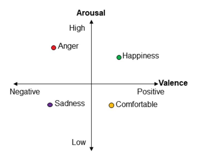
**Figure 2.** The two-dimensional model of emotions: valence–arousal plane.
### 2.2. EEG Signal Preprocessing
EEG signal preprocessing, feature extraction, and emotional state classification were performed in Python (v3.7.1) and MATLAB (vR2020b). The average number of EEG trials across datasets was 569.6 (*SD* = 423.4), including 540 for MAHNOBHCI (20 trials × 27 participants), 1280 for DEAP (40 trials × 32 participants), 150 for SEED (10 trials × 15 participants), 464 for AMIGOS (16 trials × 28 participants), and 414 for DREAMER (18 trials × 23 participants). EEG trial data were filtered using a 50/60 Hz notch and 1 Hz high-pass Butterworth filters (4th order) to remove electrical mains and DC artefact. Data were then down sampled to 128 Hz to match the sample rates across datasets, before being rereferenced to the common average, and segmented into 2-second nonoverlapping epochs. Epochs were then subjected to automatic artefact rejection to remove eye-blinks and other electrical artefacts by excluding segments with data exceeding ±100 μV. There was an average of 1046 (*SD* = 411) epochs for valence and 1036 (*SD* = 438) epochs for arousal across participants that were accepted for further analysis.
### 2.3. EEG Feature Extraction
Feature extraction refers to the process of transforming raw data into numerical features that can be processed while preserving the information in the original data set. It yields better results than applying machine learning directly to the raw data. In the emotion recognition process through EEG signals, feature extraction is the crucial part of the emotion 146
*Sensors* **2023**, *23*, 915
classification. The quality of the feature extraction will directly affect the accuracy of the emotion classification. In this study the feature extraction and analysis aimed to identify the salient EEG data that can distinguish or classify emotional states. To that end, we compared the classification performance of ten EEG feature sets that have shown reliable performance in previous emotion recognition studies [10–13,23], including Statistical, Wavelet, Fractal Dimension, Hjorth Parameters, Higher Order Spectra, Spectral Power, Entropy, Nonlinear, Connectivity, and Graph Metric features. For brevity, only the top five performing feature sets are reported in this article, including Statistical, Wavelet, Fractal Dimension, Hjorth Parameters, Higher Order Spectra features as described in Table 2. All feature sets were extracted from each channel and epoch of the preprocessed EEG data.
**Table 2.** Summary of EEG features employed in this study.
| Feature Set | Features | No. of Features |
|----------------------------|----------------------------------------------------------------------------------------------------------------------------------------------------------------------------------------------------------------------------------------------------------------------------------|-----------------|
| Statistical | Mean ( $μx$ ), Median ( $¯X$ ), Standard deviation ( $σx$ ), Skewness,
Kurtosis, Mean of absolute values of 1st difference ( $δx$ ),
Mean of absolute values of 2nd difference ( $γx$ ),
Normalized 1st difference ( $¯δx$ ), and Normalized 2nd difference ( $γ¯ x$ ) | 9 |
| Wavelet | Mean and standard deviation of the absolute values of the coefficients
in each of the 12 scales (with Morlet as mother wavelet). | 24 |
| Fractal dimension (FD) | Katz's fractal dimension (KFD), Petrosian fractal dimension (PFD),
and Higuchi's fractal dimension (HFD). | 3 |
| Hjorth parameters | Mobility ( $h1$ ), and Complexity ( $h2$ ). | 2 |
| Higher order spectra (HOS) | Bispectrum magnitude ( $BisMag$ ), Sum of logarithmic amplitudes of
Bispectrum ( $H1$ ), Sum of logarithmic amplitudes
of diagonal elements in the bispectrum ( $H2$ ), and
1st-order spectral moment of amplitudes of diagonal elements
of the bispectrum ( $H3$ ). | 4 |
#### 2.3.1. Statistical Features
Descriptive statistical measures of EEG time-series data have been used for emotion recognition in previous studies [10,11,13]. In this study, the statistical feature set includes the mean (*μX*), median (*X*¯), standard deviation (*σX*), mean of absolute values of 1st difference (*δX*), 2nd difference(*γX*), normalized 1st difference ( ¯ *δX*), and normalized 2nd difference (*γ*¯*X*) measured from the time-series data at each channel, across epochs; these features were calculated as indicated in Equations (1)–(7) below:
$$\mu_X = \frac{1}{T} \sum_{t=1}^{T} (X(t)), \tag{1}$$
$$\bar{X} = med(X(t)), (2)$$
$$\sigma_X = \sqrt{\frac{1}{T} \sum_{t=1}^{T} (X(t) - \mu_X)^2},$$
(3)
$$\delta_X = \frac{1}{T-1} \sum_{t=1}^{T-1} |(X(t+1) - X(t))|, \tag{4}$$
\gamma\_X = \frac{1}{T-2} \sum\_{t=1}^{T-2} |(X(t+2) - X(t))|, \tag{5}
$$\bar{\delta}_X = \frac{\delta_X}{\sigma_X},\tag{6}$$
147
*Sensors* **2023**, *23*, 915
$$\bar{\gamma}_X = \frac{\gamma_X}{\sigma_X} \tag{7}$$
where *X(t)* denotes the time series EEG signal and *T* represents the total number of EEG samples. In addition, we also extracted skewness, and kurtosis features from the EEG data.
#### 2.3.2. Wavelet Analysis
Wavelet transform is a popular time–frequency (TF) decomposition technique that divides the EEG signal in several approximation and details levels of wavelet coefficients corresponding to various EEG frequency ranges, while conserving the time information of the signal. Previous studies have used wavelet analysis to measure the EEG TF distribution related to emotions [13,24–26]. Here, six-level continuous wavelet transform (*CWT*) was applied using the Morlet window function to obtain wavelet coefficients of EEG bands. This mother wavelet is chosen based on its near optimal time–frequency (TF) representation characteristics [27]. Besides, Morlet wavelet is widely used in EEG-based emotion recognition studies [28,29]. For sampling rate of 128 samples/sec, we obtained 18 scales and extracted *CWT* coefficients from first 12 scales as they have frequency >1.25 Hz. Each scale frequencies are: 61.115 Hz, 43.59 Hz, 31.09 Hz, 22.17 Hz, 15.81 Hz, 11.28 Hz, 8.04 Hz, 5.74 Hz, 4.09 Hz, 2.92 Hz, 2.08 Hz, and 1.48 Hz. The equation used to compute the *CWT* coefficients from one-dimensional (1D) EEG signal data is given in Equation (8):
$$CWT(a,b) =
\int_{-\infty}^{\infty} X(t) \frac{1}{\sqrt{|a|}} \psi\left(\frac{t-b}{a}\right) dt$$
(8)
where *x(t)* denotes the time-series EEG signal in this work, *ψ* is the mother wavelet, and *a* is the scaling parameter, and *b* is the shifting parameter. Since the coefficients extracted from this frequency range are related to emotion [27–29], we computed average of the absolute values of the wavelet coefficients in each level scales as wavelet features, which is defined in Equation (9):
$$\mu_{(C_{K,\ell})} = \frac{1}{\ell} \sum_{\ell=1}^{N} |C_{K,\ell}|^2, \tag{9}$$
$$\sigma_{(C_{K,\ell})} = \sqrt{\frac{\sum \left(C(K,\ell) - \mu_{(C_{K,\ell})}\right)^2}{N}}$$
(10)
where *C*(*k*,*l*) denotes the each value of the wavelet coefficients at the *k*th decomposition level, is the number of coefficients, and *k* = 1, 2, 3··· , *N* represents the number of decomposition levels.
#### 2.3.3. Fractal Dimension
*FD* features approximate the complexity (or fractality) of the EEG times-series data providing an indication the level of self-similarity of the EEG signal across all time scales. Previously, *FD* features have shown promise for EEG-based emotion recognition [13,23,30,31]. In this study, we considered several *FD* algorithms commonly used for EEG signal analysis, namely Katz [32], Petrosian [33], and Higuchi [34]; these algorithms are explained below.
*Katz's fractal dimension (KFD)*: Katz suggested an algorithm to compute *FD* based on waveform planar curve [35], which is defined in Equation (11) as:
$$KFD = \frac{\log(L)}{\log(d)}$$
(11)
148
*Sensors* **2023**, *23*, 915
where, *d* represents the distance between the two consecutive points (curve diameter) and *L* denotes the curve length. The mean of *FD* is calculated as *KFD*, by dividing *L* and *d* by the mean distance between the locations (*a*), as shown in Equation (12):
$$KFD = \frac{\log(L)}{\log(d)} = \frac{\log(\frac{L}{a})}{\log(\frac{d}{a})} = \frac{\log(N)}{\log(N) + \log(\frac{d}{L})}$$
(12)
where *N* is the number of time samples in the EEG epoch.
*Petrosian fractal dimension (PFD)*: This algorithm converts time-series EEG signal into binary sequences [35]. The *PFD* is calculated as shown in Equation (13):
$$PFD = �rac{log(m)}{log(m) + log(�rac{m}{m + 0.4N_{\delta}})}$$
(13)
where *Nδ* denotes the number of segment pairs in the binary sequence that are not identical, and *m* represents the samples number in the segment.
*Higuchi's fractal dimension (HFD)*: Higuchi developed a method for finding *FD* directly from the original time series by decomposing into *N* samples, *X(n) = X(1), X(2), X(3)*··· *X(N)*. A new time-series signal is generated by selecting one sample after every *i*th sample, which is defined as:
$$X_{i}^{j} = X(i), X(i+j), X(i+2j), ext{...} X\left(i + \text{int}\left(\frac{N-i}{j}\right) \cdot j\right)$$
$(14)$
where *i* = 1, 2, 3, 4··· *j*. Here, *i* represents the initial time, *j* represents the internal time, and *N* represents the total number of samples. For each *i*, the length of the curve, *Li*(*j*) is represented as Equation (15), and then taken as the average value of *j* values of *Li*(*j*).
$$L_{i}(j) = �rac{\sum_{m=1}^{int\left(\frac{N-i}{j}\right)} |X(i+mj) - X(i+(m-1)j)| \cdot (n-1)}{k \cdot int\left(\frac{N-i}{j}\right)}$$
$(15)$
The HFD method is developed from the concept that the curve under consideration is fractal-like if *L*(*j*)*αj* (−*FD*) where *FD* denotes fractal dimension, and it is measured as given in Equation (16):
$$HFD = \frac{\langle L(j) \rangle}{logj} \tag{16}$$
#### 2.3.4. Hjorth Parameters
Hjorth parameters are statistical functions that explain the EEG signal characteristics in the time domain, which have also been successfully used in emotion recognition from EEG signals [10,36]. It consists of two main measures, namely mobility (*h*1), and complexity (*h*2) features [37,38], which are defined according to the following Equations (17) and (18) :
Mobility(h\_1) =
$$\sqrt{\frac{\sigma_d^2}{\sigma_{x(t)}^2}} = \frac{\sigma_d}{\sigma_{x(t)}},$$
(17)
Complexity(h\_2) =
$$\sqrt{\frac{\frac{\sigma_{dd}^2}{\sigma_d^2}}{\frac{\sigma_d^2}{\sigma_{x(t)}^2}}} = \frac{\frac{\sigma_{dd}}{\sigma_d}}{\frac{\sigma_d}{\sigma_{x(t)}}}$$
(18)
where, *x(t)* represents the time-series EEG signal with a length of *N*, *σx*(*t*) relates to the standard deviation (SD) of EEG signal, *σ*2 *x*(*t*) denotes the variance in the time-series EEG signal, *σd* denotes the SD of the 1st derivative of *x(t)*, and *σdd* denotes the SD of 2nd 149
*Sensors* **2023**, *23*, 915
derivative of *x(t)*. This activity is mobility (estimates the mean frequency), and complexity (computes the bandwidth of the signal).
### 2.3.5. Higher Order Spectra
Higher order spectra (HOS) are a spectral representation of higher order statistics that can retain the information related to deviations from Gaussianity and the degree of nonlinearity in the time-series EEG signal. Among the group of HOS features, bispectrum (*Bis*) is regarded as an effective feature for recognizing emotion from EEG signals [10,12,24]. Bispectrum depicts the Fourier Transform (FT) of the third order moment of the signal [39], calculated as shown in Equation (19).
$$Bis(f_1, f_2) = E[X(f_1) \cdot X(f_2) \cdot X^*(f_1 + f_2)] \quad (19)$$
where *X(f)* is the FT of the given signal *X(t)*, \* represents its complex conjugate, and E[·] denotes the expectation operation. In this study, bispectrum features namely, bispectrum mean magnitude (*BisMag*), and different bispectrum moments were extracted from EEG segments [40], which are computed as Equations (19)–(22):
Bispectrum magnitude, *BisMag*
$$Bis_{Mag} = \frac{1}{N} \sum_{\Omega} |Bis(f_1, f_2)|, \tag{20}$$
Bispectrum logarithmic amplitudes summation, *H*1
$$H_1 =
\sum_{\Omega} \log(|Bis(f_1, f_2)|) \quad (21)$$
Bispectrum logarithmic amplitudes of diagonal elements summation, *H*2
$$H_2 =
\sum_{\Omega} \log(|Bis(f_D, f_D)|),
(22)$$
1st order spectral moment of amplitudes of diagonal elements of the bispectrum, *H*3
$$H_3 =
\sum_{\Omega} mlog(|Bis(f_D, f_D)|)$$
(23)
where *N* is the total number of time points in the principal domain region, Ω.
### 2.4. Emotion and EEG Feature-Classification Techniques
Two classification techniques, SVM and CART, were applied and evaluated for emotional valence and arousal recognition using each EEG feature set described above, as well as a combination of all feature sets; the specific combination of a feature set (e.g., statistical) and classifier (e.g., SVM) is considered a unique feature-classification technique, which can be tested relative to other combinations. In terms of the classifiers, SVM forms a decision boundary between two classes (e.g., low vs. high valence) and attempts to increase each class distance from the decision boundary [12]. The function of kernel is to take data as input and transform it into the required form. Different SVM algorithms use different types of kernel functions. In the current study, Gaussian radial basis function (RBF) SVM (GSVM) is used due its excellent learning performance [41] in many applications including EEGbased emotion recognition [12,42,43]. CART classifiers use a minimum cost-complexity pruning technique [44]. For example, every test could consist of a linear combination of attribute values for numeric attributes. As a result, the output tree shows a hierarchy of linear models [44]. We compared the performance of four classifiers that have shown reliable classification performance in previous EEG-based emotion recognition studies [5,13], including CART, GSVM, Random forest (RF) and k-nearest neighbor (KNN). For brevity, only top two performing classifiers are reported in this paper, including CART and GSVM. 150
*Sensors* **2023**, *23*, 915
We applied Bayesian optimization technique for GSVM and CART classifiers to optimize the hyperparameters for each inner fold. For GSVM, we optimized 2 hyperparameters, namely box constrain and kernel scale. For CART, we optimized number of learning cycles, and learn rate, and minimum leaf size. Besides, we have used also random under sampling boosting for ensemble to effectively handle imbalanced data, and standardized the predictor data.
### 2.5. EEG Feature-Classification Accuracy
The accuracy of each EEG feature set-classification technique was evaluated using 4-fold cross-validation. In this approach, each participant's data was divided into 4-folds (i.e., four equal subsets of their data without overlap); 3-folds are randomly used for classifier training and the remaining fold is used as the final test for accuracy and validation. This 4-fold process is performed four times so that each fold is used as a test set, resulting in four classifier accuracy scores for each feature-classification method and participant. The mean accuracy is then computed across the 4-folds reflecting the final feature-classification accuracy per participant. This is applied separately for each dataset. To evaluate overall emotion feature-classification performance, the mean, and the SD of the final accuracy scores were computed across all participants.
### 2.6. Statistical Analysis: Comparing Feature-Classification Performance between EEG Feature Sets
Two-tailed paired-sample *t*-tests were used to evaluate whether emotion classification performance differs between feature sets. Cliff's Delta value was also computed as an additional effect-size measure of the difference between sets. It is a non-parametric effect size measure that computes the degree of difference between two groups of data (in this case, FD versus each feature set) beyond the meaning of *p*-values. Cliff's Delta range between −1 and 1, with effect sizes of −1 or 1 indicating that there is no overlap between the two groups, whereas a 0.0 indicates no difference between feature set means. Statistical significance was defined as *p*-value < 0.05. The *p*-values were corrected for multiple comparisons using Holm–Bonferroni correction.
### 2.7. EEG Scalp Topography Related to Emotion Processing
The topographic distribution of the most significant feature sets was visually inspected to consider the spatial distributions associated with high/low valence and arousal. To improve visual comparison, the features from each dataset were standardized (z-scored) and only common channels that were shared by all datasets (i.e., 14 channels) were plotted.
## 3. Experimental Results and Discussion
This section presents the classification accuracy of different feature sets and classifiers for each public EEG dataset. Higher accuracy scores are indicative of feature-classification methods that are more reliable for EEG emotion recognition. Tables 3 and 4 display the mean classification accuracy for emotional valence and arousal, respectively. Accuracy scores are shown for each feature-classification technique, including the combination of all feature sets (i.e., Combined-ALL); the highest accuracy scores within and across each dataset (i.e., Average) are highlighted in bold.
The majority of EEG feature-classification methods performed reasonably well with average classification accuracies ≥77.78% and 77.59% for valence and arousal, respectively. This is interesting as it suggests a complex relationship between 2D emotional states and many properties of the EEG signal and is consistent with the successful application of these features across previous emotion recognition studies [7,10,13]. As demonstrated by the average classification accuracy across datasets in Tables 3 and 4, the performance of EEG FD feature set was higher for classifying high/low emotional valence and arousal relative to other features when using either the GSVM or CART classifiers. These results are broadly consistent with previous research highlighting the value of FD features for detecting implicit emotional states [31,45,46]. Furthermore, the FD feature set delivered classification results
151
*Sensors* **2023**, *23*, 915
with the lowest SD of accuracy, showing that they perform more consistently than other techniques in this study; this is a valuable property, suggesting greater stability or reliability of this feature set for applied emotion recognition. This outcome is also consistent with prior research showing that the intraclass correlation coefficient (ICC) of FD features is higher for emotional state classification relative to other methods, supporting its reliability for categorizing valence and arousal [46].
**Table 3.** Emotional Valence: Mean (±SD) EEG Feature-classification accuracy (%). Bold represents the highest average accuracy scores within and across each dataset.
| Feature Set | Classifier | Dataset Name | | | | | |
|----------------------|------------|---------------|---------------|---------------|---------------|---------------|---------------|
| | | DEAP | DREAMER | MAHNOB | AMIGOS | SEED | Average |
| Combined-ALL | GSVM | 73.09 ± 0.060 | 86.56 ± 0.063 | 78.23 ± 0.080 | 76.94 ± 0.076 | 96.73 ± 0.024 | 82.31 ± 0.084 |
| | CART | 76.38 ± 0.072 | 88.44 ± 0.066 | 82.08 ± 0.081 | 78.47 ± 0.087 | 97.08 ± 0.022 | 84.49 ± 0.075 |
| Statistical | GSVM | 69.62 ± 0.066 | 83.74 ± 0.064 | 75.47 ± 0.077 | 74.47 ± 0.082 | 96.14 ± 0.035 | 79.89 ± 0.093 |
| | CART | 75.02 ± 0.086 | 88.26 ± 0.067 | 81.67 ± 0.097 | 78.19 ± 0.087 | 97.01 ± 0.020 | 84.03 ± 0.078 |
| Wavelet | GSVM | 69.11 ± 0.064 | 82.10 ± 0.075 | 71.94 ± 0.079 | 72.34 ± 0.070 | 93.39 ± 0.047 | 77.78 ± 0.089 |
| | CART | 77.34 ± 0.066 | 87.99 ± 0.066 | 82.57 ± 0.082 | 79.12 ± 0.084 | 96.78 ± 0.023 | 84.76 ± 0.070 |
| Fractal dimension | GSVM | 75.69 ± 0.065 | 83.94 ± 0.065 | 80.91 ± 0.078 | 76.83 ± 0.084 | 96.40 ± 0.030 | 82.75 ± 0.074 |
| | CART | 78.18 ± 0.079 | 87.59 ± 0.067 | 83.98 ± 0.087 | 79.07 ± 0.084 | 96.50 ± 0.030 | 85.06 ± 0.066 |
| Hjorth parameters | GSVM | 73.23 ± 0.068 | 82.20 ± 0.066 | 78.82 ± 0.069 | 71.57 ± 0.067 | 96.32 ± 0.023 | 80.43 ± 0.088 |
| | CART | 70.52 ± 0.063 | 80.86 ± 0.065 | 75.33 ± 0.071 | 70.21 ± 0.070 | 94.25 ± 0.037 | 78.23 ± 0.089 |
| Higher order spectra | GSVM | 73.78 ± 0.073 | 83.31 ± 0.076 | 79.39 ± 0.081 | 72.23 ± 0.086 | 96.83 ± 0.028 | 81.11 ± 0.088 |
| | CART | 72.18 ± 0.076 | 83.68 ± 0.069 | 78.27 ± 0.087 | 72.98 ± 0.082 | 95.66 ± 0.037 | 80.56 ± 0.086 |
**Table 4.** Emotional Arousal: Mean (±SD) EEG Feature-classification accuracy (%). Bold represents the highest average accuracy scores within and across each dataset.
| Feature
Set | Classifier | Dataset Name | | | | |
|----------------------|------------|---------------|---------------|---------------|---------------|---------------|
| | | DEAP | DREAMER | MAHNOB | AMIGOS | Average |
| Combined-ALL | GSVM | 75.83 ± 0.072 | 90.35 ± 0.072 | 80.55 ± 0.081 | 79.49 ± 0.093 | 81.56 ± 0.053 |
| | CART | 78.82 ± 0.076 | 92.02 ± 0.065 | 83.21 ± 0.082 | 81.00 ± 0.092 | 83.76 ± 0.050 |
| Statistical | GSVM | 72.51 ± 0.085 | 88.92 ± 0.072 | 77.46 ± 0.084 | 77.10 ± 0.103 | 79.00 ± 0.060 |
| | CART | 77.38 ± 0.092 | 91.76 ± 0.068 | 83.72 ± 0.084 | 80.94 ± 0.087 | 83.45 ± 0.053 |
| Wavelet | GSVM | 71.60 ± 0.079 | 87.62 ± 0.089 | 75.65 ± 0.095 | 77.15 ± 0.096 | 78.01 ± 0.059 |
| | CART | 78.83 ± 0.077 | 91.60 ± 0.067 | 84.14 ± 0.082 | 81.20 ± 0.087 | 83.94 ± 0.048 |
| Fractal dimension | GSVM | 77.48 ± 0.072 | 88.99 ± 0.074 | 82.80 ± 0.079 | 79.10 ± 0.088 | 82.09 ± 0.044 |
| | CART | 79.90 ± 0.086 | 91.60 ± 0.067 | 85.58 ± 0.085 | 81.11 ± 0.087 | 84.55 ± 0.045 |
| Hjorth parameters | GSVM | 75.62 ± 0.069 | 87.02 ± 0.083 | 80.70 ± 0.075 | 75.28 ± 0.099 | 79.66 ± 0.047 |
| | CART | 73.14 ± 0.071 | 86.07 ± 0.085 | 76.94 ± 0.080 | 74.21 ± 0.107 | 77.59 ± 0.050 |
| Higher order spectra | GSVM | 75.83 ± 0.079 | 88.35 ± 0.082 | 81.13 ± 0.083 | 76.77 ± 0.091 | 80.52 ± 0.049 |
| | CART | 75.36 ± 0.081 | 88.69 ± 0.081 | 79.62 ± 0.086 | 76.79 ± 0.098 | 80.11 ± 0.051 |
N.B. The SEED dataset is not listed as it did not record arousal data.
Another important finding of the present study is that CART classifiers performed better for EEG emotion recognition compared to GSVM. Using the FD feature set, we achieved the highest mean classification accuracy (average across the five datasets) for valence and arousal as 85.06% and 84.55%, with CART classifier (hereafter named as FD-CART). This
152
*Sensors* **2023**, *23*, 915
was found to be the case across all datasets utilized in this study and is in line with previous research supporting the utility of CART for emotion recognition [47,48]. For that reason, we focus on reporting feature set outcomes utilizing the CART classifier in subsequent sections. Figure 3 shows the box plot of the top three feature set (fractal dimension, wavelet transform, and statistical features) accuracies using CART on each dataset. The plot visually displays the distribution of classification accuracies across each subject and illustrates that the reliability of selected EEG feature set for applied emotion recognition. Table 5 summarizes the statistical results of two-tailed paired *t*-tests comparing CART classification performance between different feature sets. The *t*-test outcomes (*p*-values) and Cliff's Delta effect size also demonstrate that FD features have significantly higher accuracy than other feature sets, confirming the descriptive observations in Tables 3 and 4.
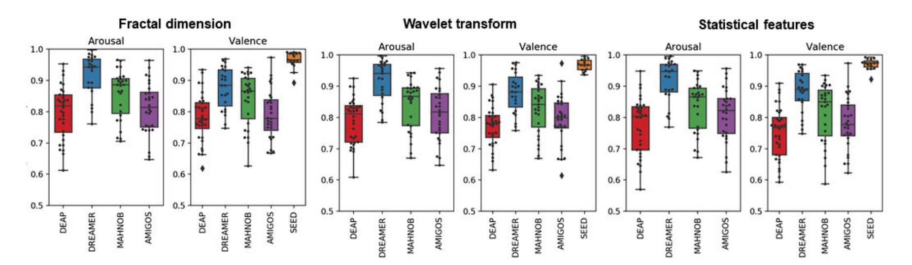
**Figure 3.** Top three feature sets. Boxplot of CART accuracy on each DEAP, DREAMER, MAHNOB, AMIGOS and SEED emotion dataset. *X*-axis represents the dataset name. *Y*-axis indicates the classification accuracy. Black dot in the figure represents average classification accuracy of each participant across 4-folds.
Table 5 shows the statistical results of two-tailed paired *t*-test of CART classification performances among different feature sets. From the *p*-value, it is clear that the results from the FD are statistically different (*p*-value < 0.05) from other feature sets listed in the table, including the combination of features. Table 5 also provides the mean difference effect size for paired samples based on Cliff's Delta. From the Cliff's Delta, it is apparent that, across the five datasets, the emotional state classification accuracy with FD feature set is more accurate on average. However, it is not always the most accurate in each individual case.
The present research utilized a data-driven approach for identifying EEG features that are optimal for emotion detection, thus while FD clearly demonstrates the best performance, it is currently unclear why this feature set is the most effective. Further research is needed to investigate this matter; however, considering our results and the prior literature, we speculate that methodological (technical) and/or functional reasons could explain why FD features are most effective for emotion recognition. In terms of methodology, FD features are nonlinear complexity estimators and calculated over short time-periods, are robust to noise, and do not require any prior transformation of the time series [46,49]. This differs to other methods (e.g., wavelet, statistical) and is beneficial for emotion recognition. At a functional level, fractality indicates whether the EEG signal is synchronous or repetitive over different time scales (i.e., similar patterns occur over shorter and longer intervals), representing the nonlinear complexity of underlying brain activity [50]. As explained by Zappasodi et al. [50] complexity is considered to reflect efficient neuronal functioning, varying between randomness and constant periodicity; with the extremes related to disfunction and difficulty shifting between brain states. From this viewpoint, we can speculate that different emotional states are associated with unique levels of signal complexity, with high/low valence and arousal leading to important shifts in network complexity on a spectrum. This is consistent with the idea that emotions can drive mental (and neuronal)
153
*Sensors* **2023**, *23*, 915
states associated with more or less lability and/or cognitive flexibility (e.g., [51]). FD may provide a relevant and effective means to model those functional differences, which are not captured in other EEG measures of 2D emotional states.
**Table 5.** Statistical results (*p*-values effect size) of two-tailed paired *t*-test of CART classification performances among different feature sets.
| Condition | p -Value | | Cliff's Delta Effect Size | |
|-----------------------------|-----------------|--------------|---------------------------|---------|
| | Arousal | Valence | Arousal | Valence |
| FD vs. Wavelet | 3.31 × 10⁻³ | 3.53 × 10⁻² | 0.045 | 0.022 |
| FD vs. Statistical | 6.85 × 10⁻⁸ | 1.31 × 10⁻⁹ | 0.063 | 0.061 |
| FD vs. Hjorth Parameters | 2.13 × 10⁻¹⁹ | 1.22 × 10⁻²¹ | 0.397 | 0.420 |
| FD vs. Higher order spectra | 3.01 × 10⁻¹⁹ | 1.53 × 10⁻²¹ | 0.261 | 0.277 |
| Combined-ALL | 3.93 × 10⁻⁴ | 1.25 × 10⁻³ | 0.058 | 0.045 |
Effect size based on Cliff's Delta. FD—Fractal dimension.
The topography of FD features (i.e., KFD, PFD, and HFD) associated with high or low valence are plotted in Figure 4. The grand mean (GM) head maps calculated across datasets for KFD suggest that higher (i.e., more positive) valence was associated with less complexity (fractality) at frontal electrode sites, particularly over the left hemisphere, relative to periods of low valence. This pattern is somewhat consistent with the GM topography of PFD, which suggests higher valence is related to lower complexity at frontal, temporal, and occipital electrode sites. GM HFD indicates a slightly different pattern, with higher valence linked to relatively higher complexity at the most frontal EEG channels, but lower complexity over left frontocentral regions. In general, these results suggest that states of higher valence are related to less EEG complexity over frontal regions. However, this is not always consistent within datasets, and given the limited sites these topographic findings should be considered tentatively.
The topography of FD features (i.e., KFD, PFD, and HFD) associated with high or low arousal are plotted in Figure 5. The GM headmaps for KFD suggest that higher arousal is related to lower complexity at frontal and temporal sites over the left hemisphere. GM PFD is shows a similar spatial distribution for high and low arousal, with lower complexity at left frontocentral sites and temporoparietal sites relative to other scalp regions, and this pattern is stronger in periods of high arousal. GM HFD shows the opposite pattern compared to PFD. These GM topographic distributions are somewhat consistent with those shown for valence, with higher arousal broadly associated with lower complexity over the left hemisphere. However, it is important to note that these topographic interpretations are based only on visual inspection with limited channels. It is also apparent that these GM spatial distributions of FD features are not completely consistent across all datasets. For that reason, these topographic results should only be used as a tentative guide for research interested in FD distribution relative to emotional states or the optimal location for electrodes to facilitate EEG emotion recognition. For more definitive outcomes future research involving more EEG channels is needed.
Table 6 provides a comparison to other studies in the literature that have utilized more than one dataset to validate their methods. As the AMIGOS and DREAMER emotion datasets were only lately released, there are only limited comparative studies and hence, for comparison, baseline evaluation work also included in Table 5. Siddharth et al. [52] utilized RGB topographic maps computed from power spectral density (PSD) features using bicubic interpolation and assessed binary classification (low/high) for valence and arousal emotion using DEAP, DREAMER, MANHOB, and AMIGOS . They achieved results 71.09–83.02% for valence and 72.58–80.42% for arousal emotion recognition. In another study, Li et al. [53] suggested an approach that generates spatial maps from EEG signals and combined graph regularized extreme learning machine (GRELM) with SVM for recognizing emotions. They obtained an accuracy of 62.005–88.00% for valence emotion on DEAP and SEED emotion datasets. In the recent study, Topic and Russo [19] demonstrated a hybrid
154
*Sensors* **2023**, *23*, 915
deep learning approach using holographic and topographic feature maps for emotion recognition using EEG signals. In this approach, they introduced EEG-topography in which they utilized the spatial and spectral information and performed classification of valence and arousal on DEAP, DREAMER, AMIGOS and SEED datasets. They reported 76.61–88.45% and 77.72–90.54% for valence and arousal emotion recognition, respectively. The AMIGOS emotion dataset [17] authors achieved the classification accuracy of 57.60% for valence state and 59.20% for arousal state using power spectral density (PSD) EEG features. Similarly, the researchers of the DREAMER dataset [15] achieved emotion recognition accuracy of 62.49% and 62.17% for valence and arousal, respectively. From all these studies, we can see that the identified FD feature set performs better than comparable methods previously reported for both affective states consistently in all the five datasets. This demonstrates the effectiveness of fractal dimension features combined with CART classifier for emotion recognition using EEG signals.
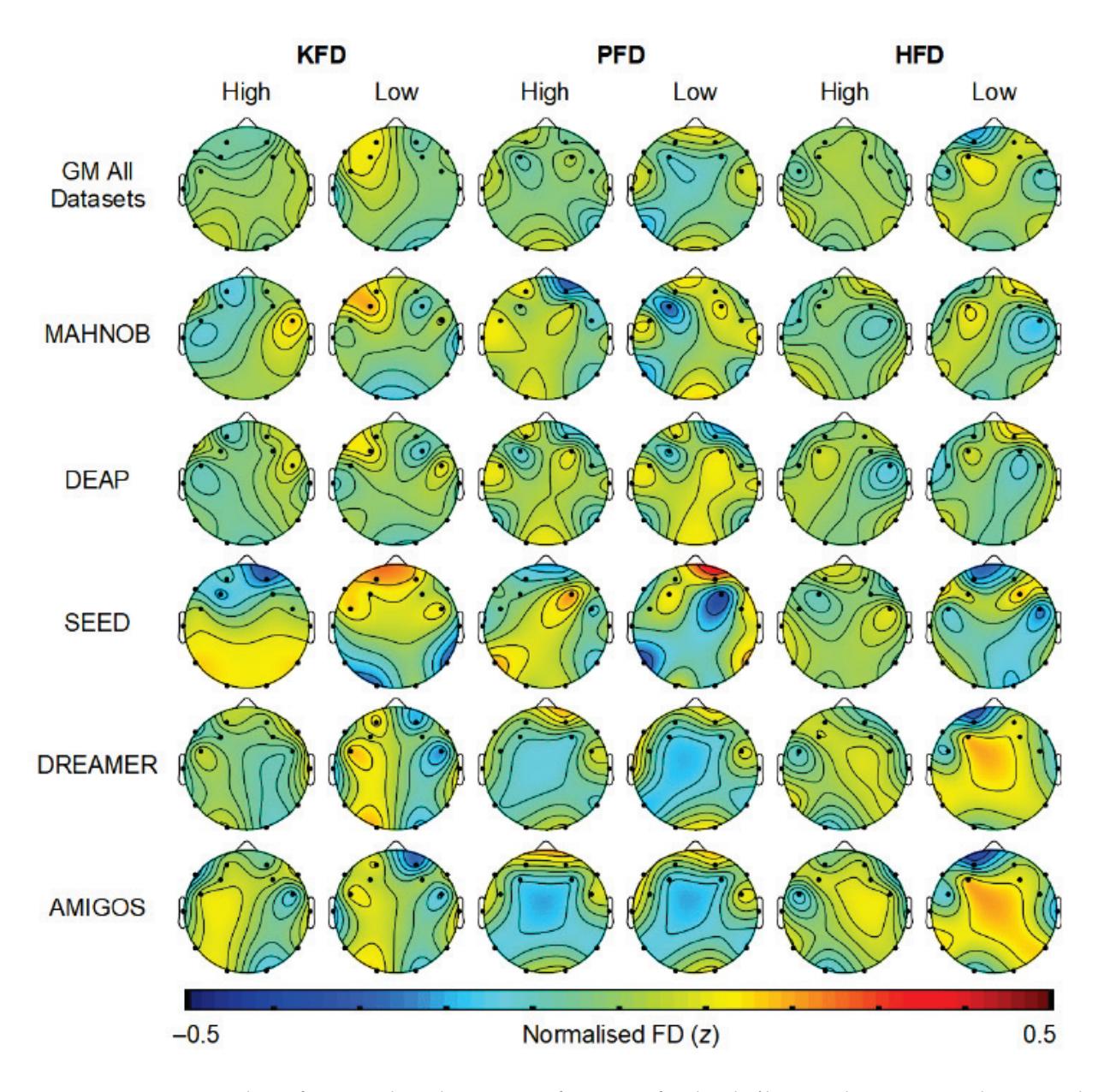
**Figure 4.** Topography of normalized EEG FD features for high/low valence. GM denotes the grand mean of each FD feature across all the datasets. KFD—Katz's fractal dimension, PFD—Petrosian fractal dimension, HFD—Higuchi's fractal dimension.
155
*Sensors* **2023**, *23*, 915
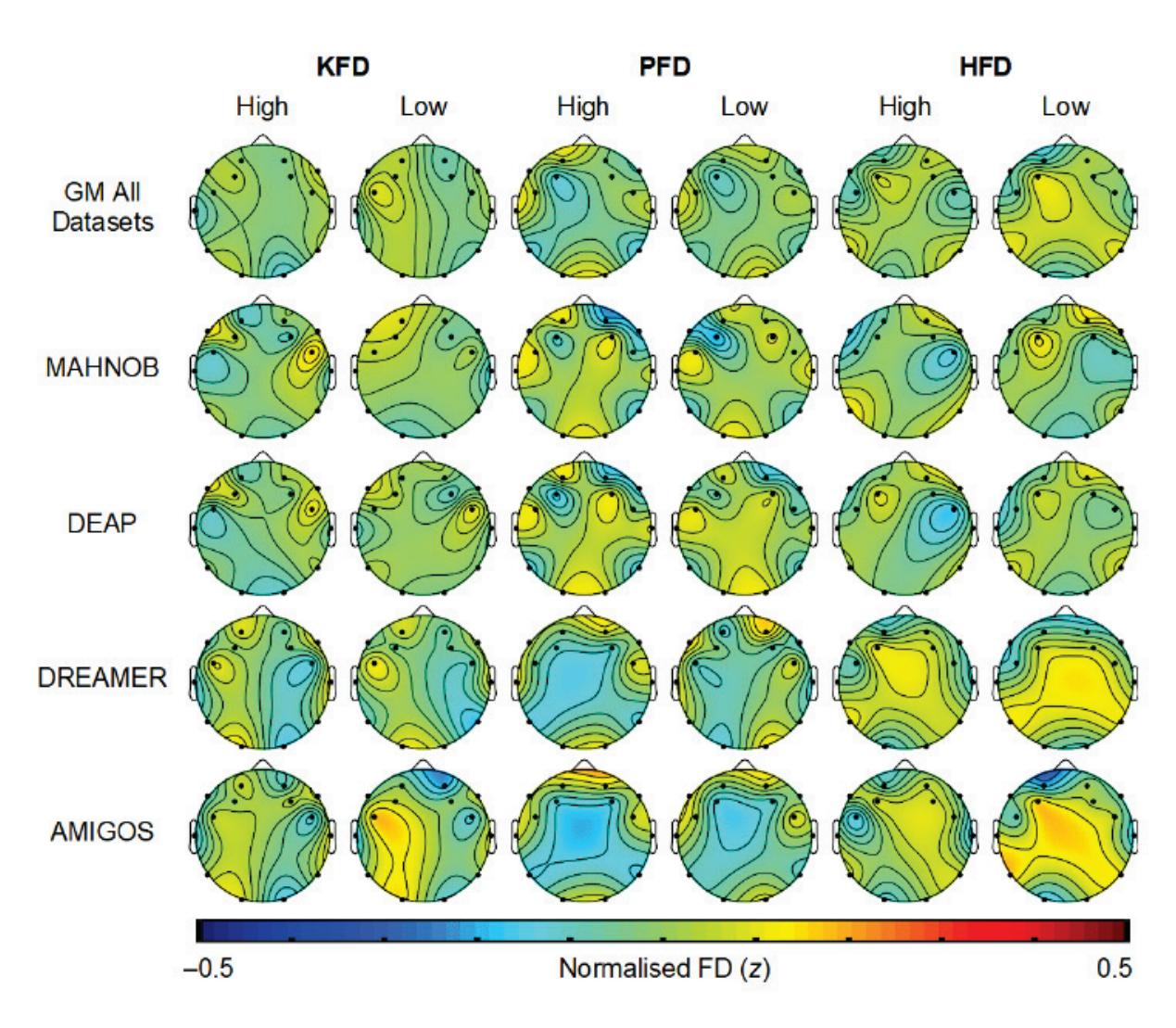
**Figure 5.** Topography of normalized EEG FD features for high/low arousal. SEED dataset does not have arousal class. GM denotes the grand mean of FD each feature across all the datasets.KFD-Katz's fractal dimension, PFD-Petrosian fractal dimension, HFD-Higuchi's fractal dimension.
**Table 6.** Comparison with other studies in the literature.
| Research
Study | Features Employed
Classification Method | Best Accuracy (%) Achieved | | | | |
|--------------------------|--------------------------------------------|----------------------------|----------|---------|---------|---------|
| | | DEAP | DREAMER | MAHNOB | AMIGOS | SEED |
| Topic and Russo, [19] | HOLOfm | V:76.61 | V:88.20 | - | V:87.39 | V:88.45 |
| | CNN-SVM | A:77.72 | A:90.43 | - | A:90.54 | A: - |
| Topic and Russo, [19] | TOPOfm | V:76.30 | V:81.96 | - | V:80.63 | V:70.37 |
| | CNN-SVM | A:76.54 | A:84.92 | - | A:85.75 | A: - |
| Siddharth et al. [52] | RGB colored image | V:71.09 | V:78.99 | V:80.77 | V:83.02 | - |
| | CNN-ELM | A:72.58 | A:79.23 | A:80.42 | A:79.13 | - |
| Li et al. [53] | Spatial map | V:62.00 | - | - | - | V:88.00 |
| | GRELM-SVM | A: - | - | - | - | A: - |
| Katsigiannis et al. [15] | PSD | - | V: 62.49 | - | - | - |
| | SVM | - | A:62.17 | - | - | - |
| Miranda et al. [17] | PSD, SPA | - | - | - | V:57.60 | - |
| | SVM | - | - | - | A:59.20 | - |
| This study | FD-CART | V:78.18 | V:87.59 | V:83.98 | V:79.07 | V:96.50 |
| | | A:79.90 | A:91.60 | A:85.58 | A:81.11 | A: - |
"-" means that this experiment was not in this research. A—Arousal, CNN—Convolutional Neural Network, ELM—Extreme Learning Machine; GELM—Graph regularized Extreme Learning Machine, HOLO-FM— Holographic Feature Maps, PSD—Power spectral Density, SPA—Spectral Power Asymmetry, SVM—Support Vector Machine, TOPO-FM—Topographic Feature Maps, V—Valence.
## 4. Conclusions
In this work, we present a comparative analysis on different feature extraction methods using multichannel EEG recordings for the creation of a reliable emotional state recognition system. A comprehensive set of features (statistical, FD, Hjorth parameters, HOS, 156
*Sensors* **2023**, *23*, 915
and wavelet transform features) were obtained from the EEG signals. We conducted a quantitative comparison of feature extraction techniques with two different classifiers, GSVM, and CART. The emotion EEG datasets namely, DEAP, DREAMER, MAHNOB, AMIGOS and SEED were used to assess the performance of the study. The findings revealed that FD feature set are the most sensitive feature metric in distinguishing emotions categorized in terms of high/low valence and arousal. The FD-CART feature-classification method tested in this study achieves an overall best mean accuracy of 86.79% and 84.55% for binary classification of valence, and arousal, respectively, using all features in the FD set. Our results suggest that the fractality of the EEG time-domain data has a substantial role and is more reliable for emotional state recognition. This might result in the creation of an effective online framework for extracting EEG features and the development of a real-time human computer interactive system for emotional state recognition.
The study comes with two limitations. Firstly, it would be interesting to explore deep learning classifiers as an alternative for CART and SVM. In recent years, convolutional layers of deep neural networks have been found successful in EEG-based classification of emotion [54,55]. It was not feasible to explore this approach here due to lack of data. However, integrating deep learning with the present research may be a fruitful direction for further work in EEG emotion recognition. Secondly, though subject-dependent cross-validation approach is carried out, building a truly subject-independent (e.g., leave-one-subject-out) system would be more reliable and scalable. In the future, we will extend this approach to subject independent cross-validation (e.g., leave-one-subject-out) with emotional state categorization in three-dimensional space, i.e., the valence-arousal-dominance emotional model. In addition, we also intend to investigate the FD-CART feature-classification method on the combined emotion EEG datasets for training, validation, and evaluation purposes.
**Author Contributions:** Conceptualization, R.Y., P.T. and J.T.; methodology, R.Y., P.T. and J.T.; investigation, P.T., R.Y., J.T. and J.F.; writing—original draft preparation, R.Y. and J.F.; writing—review and editing, R.Y., J.F., P.T., J.T. and F.A.; project administration, R.Y.; funding acquisition, R.Y. All authors have read and agreed to the published version of the manuscript.
**Funding:** This research was financed by the Singapore Ministry of Education (MOE) through the Education Research Funding Programme (ERFP) (Grant No: PG 03/21 YR), which was overseen by the National Institute of Education (NIE), Nanyang Technological University (NTU), Singapore.
**Institutional Review Board Statement:** Not applicable.
**Informed Consent Statement:** Not applicable.
**Data Availability Statement:** Not applicable.
**Acknowledgments:** The authors would like to thank the research teams who collected and made the datasets available publicly and for granting access to the datasets.
**Conflicts of Interest:** The authors declare no conflict of interest.
#### Abbreviations
The following abbreviations are used in this manuscript:
CART Classification and Regression Tree DWT Discrete Wavelet Transform DEAP Dataset for Emotion Analysis using Physiological signals ECG Electrocardiogram EEG Electroencephalogram EDA Electrodermal Activity EMG electromyogram ERP Event Related Potential
ERO Event Related Oscillation FD Fractal Dimension
GM Grand Mean
157
*Sensors* **2023**, *23*, 915
| Abbreviation | Full Name |
|--------------|-------------------------------------------------------|
| GSVM | Gaussian Radial Basis Function Support Vector Machine |
| GSR | Galvanic Skin Resistance |
| HFD | Higuchi's fractal dimension |
| HOC | Higher Order Crossing |
| HOS | Higher Order Spectra |
| KFD | Katz's Fractal Dimension |
| KNN | K-Nearest Neighbor |
| PFD | Petrosian fractal dimension |
PNS Peripheral Nervous System RF Random Forest RR Respiration Rate SD Standard Deviation SVM Support Vector Machine
#### References
- 1. Shu, L.; Xie, J.; Yang, M.; Li, Z.; Li, Z.; Liao, D.; Xu, X.; Yang, X. A Review of Emotion Recognition Using Physiological Signals. *Sensors* **2018**, *18*, 2074. [CrossRef] [PubMed]
- 2. Egger, M.; Ley, M.; Hanke, S. Emotion recognition from physiological signal analysis: A review. *Electron. Notes Theor. Comput. Sci.* **2019**, *343*, 35–55. [CrossRef]
- 3. Ko, B.C. A brief review of facial emotion recognition based on visual information. *Sensors* **2018**, *18*, 401. [CrossRef] [PubMed]
- 4. Wani, T.M.; Gunawan, T.S.; Qadri, S.A.A.; Kartiwi, M.; Ambikairajah, E. A comprehensive review of speech emotion recognition systems. *IEEE Access* **2021**, *9*, 47795–47814. [CrossRef]
- 5. Liu, H.; Zhang, Y.; Li, Y.; Kong, X. Review on emotion recognition based on electroencephalography. *Front. Comput. Neurosci.* **2021**, *15*, 758212. [CrossRef]
- 6. Schaaff, K.; Schultz, T. Towards emotion recognition from electroencephalographic signals. In Proceedings of the 3rd International Conference on Affective Computing and Intelligent Interaction and Workshops (ACII 2009), Amsterdam, The Netherlands, 10–12 September 2009.
- 7. Petrantonakis, P.C.; Hadjileontiadis, L.J. Emotion recogntion from brain signals using hybrid adaptive filtering and higher order crossings analysis. *IEEE Trans. Affect. Comput.* **2010**, *1*, 81–96. [CrossRef]
- 8. Frantzidis, C.A.; Bratsas, C.; Papadelis, C.L.; Konstantinidis, E.; Pappas, C.; Bamidis, P.D. Toward emotion aware computing:An integrated approach using multichannel neurophysiological recordings and affective visual stimuli. *IEEE Trans. Inf. Technol. Biomed*. **2010**, *14*, 589–597. [CrossRef]
- 9. Hadjidimitriou, S.K.; Hadjileontiadis, L.J. Toward an EEG-based recognition of music liking using time-frequency analysis. *IEEE Trans. Biomed. Eng*. **2012**, *59*, 3498–3510. [CrossRef]
- 10. Jenke, R.; Peer, A.; Buss, M. Feature extraction and selection for emotion recogntion from EEG. *IEEE Trans. Affect. Comput.* **2014**, *5*, 327–339. [CrossRef]
- 11. Liu, Y.; Sourina, O. Real-time subject-dependent eeg-based emotion recognition algorithm. In *Transactions on Computational Science XXIII*; Springer: Berlin/Heidelberg, Germany, 2014; pp. 199–223.
- 12. Yuvaraj, R.; Murugappan, M.; Norlinah, M.I.; Sundaraj, K.; Omar, M.I.; Khairiyah, M.; Palaniappan, R. Optimal set of EEG features for emotional state classification and trajectory visualization in Parkinsosn's disease. *Int. J. Psychophysiol.* **2014**, *94*, 482–495. [CrossRef]
- 13. Nawaz, R.; Cheah, K.H.; Nisar, H.; Yap, V.V. Comparison of different feature extraction methods for EEG-based emotion recognition. *Biocybern. Biomed. Eng.* **2020**, *40*, 910–926. [CrossRef]
- 14. Koelstra, S.; Soleymani, M.; Lee, J.-S.; Yazdani, A.; Ebrahimi, T.; Pun, T.; Nijholt, A.; Patras, I. DEAP: A Database for Emotion Analysis ;Using Physiological Signals. *IEEE Trans. Affect. Comput.* **2012**, *3*, 18–31. [CrossRef]
- 15. Katsigiannis, S.; Ramzan, N. DREAMER: A Database for Emotion Recognition Through EEG and ECG Signals From Wireless Low-cost Off-the-Shelf Devices. *IEEE J. Biomed. Health Inform.* **2018**, *22*, 98–107. [CrossRef]
- 16. Soleymani, M.; Lichtenauer, J.; Pun, T.; Pantic, M. A Multimodal Database for Affect Recognition and Implicit Tagging. *IEEE Trans. Affect. Comput.* **2012**, *3*, 42–55. [CrossRef]
- 17. Miranda-Correa, J.A.; Abadi, M.K.; Sebe, N.; Patras, I. AMIGOS: A Dataset for Affect, Personality and Mood Research on Individuals and Groups. *IEEE Trans. Affect. Comput.* **2017**, *12*, 479–493. [CrossRef]
- 18. Zheng, W.L.; Lu, B.L. Investigating critical frequency bands and channels for EEG-based emotion recognition with deep neural networks. *IEEE Trans. Auton. Ment. Dev.* **2015**, *7*, 162–175. [CrossRef]
- 19. Topic, A.; Russo, M. Emotion recognition based on EEG feature maps through deep learning network. *Int. J Eng. Sci. Technol.* **2021**, *24*, 1441–1454. [CrossRef]
- 20. Li, X.; Song, D.; Zhang, P.; Zhang, Y.; Hou, Y.; Hu, B. Exploring EEG features in cross-subject emotion recognition. *Front. Neurosci*. **2018**, *12*, 162. [CrossRef]
- 21. Lan, Z.; Sourina, O.; Wang, L.; Scherer, R.; Müller-Putz, G.R. Domain adaptation techniques for EEG-based emotion recognition: A comparative study on two public datasets. *IEEE Trans. Cogn. Dev. Syst.* **2018**, *11*, 85–94. [CrossRef]
158
*Sensors* **2023**, *23*, 915
- 22. Posner, J.; Russell, J.A.; Peterson, B.S. The circumplex model of affect: An integrative approach to affective neuroscience, cognitive development, and psychopathology. *Dev. Psychopathol.* **2005**, *17*, 715–734. [CrossRef] [PubMed]
- 23. Liu, J.; Meng, H.; Li, M.; Zhang, F.; Qin, R.; Nandi, A.K. Emotion detection from EEG recordings based on supervised and unsupervised dimension reduction. *Concurr. Comput.* **2018**, *30*, 1–13. [CrossRef]
- 24. Piho, L.; Tjahjadi, T. A mutual information based adaptive windowing of informative EEG for emotion recognition. *IEEE Trans. Affect. Comput.* **2018**, *11*, 722–735. [CrossRef]
- 25. Garg, A.; Kapoor, A.; Bedi, A.K.; Sunkaria, R.K. Merged LSTM Model for emotion classification using EEG signals. In Proceedings of the International Conference on Data Science and Engineering (ICDSE), Patna, India, 26–28 September 2019.
- 26. Putra, A.E.; Atmaji, C.; Ghaleb, F. EEG-Based Emotion Classification Using Wavelet Decomposition and K-Nearest Neighbor. In Proceedings of the 4th International Conference on Science and Technology (ICST), Yogyakarta, Indonesia, 7–8 August 2018.
- 27. Wang, X.W.; Nie, D.; Lu, B.L. Emotional state classification from EEG data using machine learning approach. *Neurocomputing* **2013**, *129*, 94–106. [CrossRef]
- 28. Taran, S.; Bajaj, V. Emotion recognition from single-channel EEG signals using a two-stage correlation and instantaneous frequency-based filtering method. *Comput. Programs Biomed.* **2019**, *173*, 157–165. [CrossRef] [PubMed]
- 29. Bajaj, V.; Pachori, R.B. Human Emotion Classification from EEG Signals Using Multiwavelet Transform. In Proceedings of the International Conference on Medical Biometrics, Shenzhen, China, 30 May–1 June 2014; pp. 125–130.
- 30. Avramidis, K.; Zlatintsi, A.; Garoufis, C.; Maragos, P. Multiscale Fractal Analysis on EEG Signals for Music-Induced Emotion Recognition. Available online: https://arxiv.org/abs/2010.16310 (accessed on 20 January 2022).
- 31. Liu, Y.; Sourina, O. Real-Time Fractal-Based Valence Level Recognition from EEG. In *Transactions on Computational Science XVIII*; Gavrilova, M.L., Tan, C.J.K., Kuijper, A., Eds.; Lecture Notes in Computer Science; Springer: Berlin/Heidelberg, Germany, 2013; p. 7848.
- 32. Katz, M.J. Fractals and the analysis of waveforms. *Comput. Biol. Med*. **1998**, *18*, 145–156. [CrossRef]
- 33. Hatamikia, S.; Nasrabadi, A.M. Recognition of emotional states induced by music videos based on nonlinear feature extraction and SOM classification. In Proceedings of the 21st Iranian Conference on Biomedical Engineering (ICBME), Tehran, Iran, 26–28 November 2014; pp. 333–337.
- 34. Higuchi, T. Approach to an irregular time series on the basis of the fractal theory. *Phys. D* **1988**, *31*, 277–283. [CrossRef]
- 35. Garcia-Martinez, B.; Martinez-Rodrigo, A.; Alcaraz, R.; Fernandez-Caballero, A. A Review on nonlinear methods using electroencephalographic recordings for emotion recognition. *IEEE Trans. Affect. Comput.* **2019**, *10*, 1–20. [CrossRef]
- 36. Mehmood, R.M.; Du, R.; Lee, H.J. Optimal feature selection and deep learning ensembles method for emotion recognition from human brain EEG sensors. *IEEE Access*. **2017**, *5*, 14797–14806. [CrossRef]
- 37. Hjorth, B. EEG analysis based on time domain properties. *Electroencephalogr. Clin. Neurophysiol*. **1970**, *29*, 306–310. [CrossRef]
- 38. Hjorth, B. The physical significance of time domain descriptors in EEG analysis. Electroencephalogr. *Clin. Neurophysiol*. **1973**, *34*, 312–325.
- 39. Hosseini, S.A. Classification of brain activity in emotional states using HOS analysis. *Int. J Image Graph. Signal Process.* **2012**, *1*, 21–27. [CrossRef]
- 40. Yuvaraj, R.; Acharya, U.; Hagiwara, Y. A novel Parkinson's Disease Diagnosis Index using higher-order spectra features in EEG signals. *Neural Comput. Appl.* **2016**, *30*, 1225–1235. [CrossRef]
- 41. Yang, J.; Wu, Z.; Peng, K.; Okolo, P.N.; Zhang, W.; Zhao, H.; Sun, J. Parameter selection of Gaussian kernel SVM based on local density of training set. *Inverse. Probl. Sci. Eng.* **2021**, 29, 536–548. [CrossRef]
- 42. Mehmood, R.M.; Lee, H.J. Emotion classification of EEG brain signal using SVM and KNN. In Proceedings of the International Conference on Multimedia & Expo Workshops (ICMEW), Turin, Italy, 29 June–3 July 2015.
- 43. Satyanarayana, K.N.V.; Shankar, T.; Poojita, G.; Vinay, G.; Amaranadh, H.N.S.V.l.S.; Babu, A.G. An Approach to EEG based Emotion Identification by SVM classifier. In Proceedings of the 6th International Conference on Computing Methodologies and Communication (ICCMC), Erode, India, 29–31 March 2022.
- 44. Witten, I.H.; Frank, E.; Hall, M.A. *Data Mining: Practical Machine Learning Tools and Techniques*; Elsevier: Burlington, NJ, USA, 2011.
- 45. Liu, Y.; Sourina, O.; Nguyen, M.K. Real time EEG-based emotion recognition and its applications. *Trans. Comput. Sci.* **2011**, *6670*, 256–277.
- 46. Lan, Z.; Sourina, O.; Wang, L.; Liu, Y. Real-time EEGbased emotion monitoring using stable features. *Visual Comput.* **2016**, *32*, 347–358. [CrossRef]
- 47. Thomas, J.; Jin, J.; Thangavel, P.; Bagheri, E.; Yuvaraj, R.; Dauwels, J.; Rathakrishnan, R.; Halford, J.J.; Cash, S.S.; Westover, B. Automated Detection of Interictal Epileptiform Discharges from Scalp Electroencephalograms by Convolutional Neural Networks. *Int. J. Neural Syst.* **2020**, *30*, 2050030. [CrossRef]
- 48. Jukic, S.; Saracevic, M.; Subasi, A.; Kevric, J. Comparison of Ensemble Machine Learning Methods for Automated Classification of Focal and Non-Focal Epileptic EEG Signals. *Mathematics* **2020**, *8*, 1481. [CrossRef]
- 49. Ruiz-Padial, E.; Ibáñez-Molina, A.J. Fractal dimesion of EEG signals and heart dynamics in discrete emotional states. *Biol. Psychol.* **2018**, *137*, 42–48. [CrossRef]
- 50. Zappasodi, F.; Olejarczyk, E.; Marzetti, L.; Assenza, G.; Pizzella, V.; Tecchio, F. Fractal dimension of EEG activity senses neuronal impairment in acute stroke. *PLoS ONE* **2014**, *9*, e100199. [CrossRef]
159
*Sensors* **2023**, *23*, 915
- 51. Plessow, F.; Fischer, R.; Kirschbaum, C.; Goschke, T. Inflexibly focused under stress: Acute psychosocial stress increases shielding of action goals at the expense of reduced cognitive flexibility with increasing time lag to the stressor. *J. Cogn. Neurosci.* **2011**, *23*, 3218–3227. [CrossRef]
- 52. Siddharth, S.; Jung, T.-P.; Sejnowski, T.J. Utilizing deep learning towards multi-modal bio-sensing and vision-based affective computing. *arXiv* **2019**, arXiv:1905.07039.
- 53. Li, P.; Liu, H.; Si, Y.; Li, C.; Li, F.; Zhu, X.; Huang, X.; Zeng, Y.; Yao, D.; Zhang, Y.; et al. EEG based emotion recognition by combining functional connectivity network and local activations. *IEEE Trans. Biomed. Eng.* **2019**, *66*, 2869–28881. [CrossRef]
- 54. Cui, H.; Liu, A.; Zhang, X.; Chen, X.; Wang, K.; Chen, X. EEG-based Emotion Recognition using an End-to-End Regional-Asymmetric Convolutional Neural Network. *Knowl. Based. Systs.* **2020**, *205*, 106243. [CrossRef]
- 55. Han, Z.; Chang, H.; Zhou, X.; Wang, J.; Wang, L.; Shao, Y. E2ENNet: An End-to-End Neural Network for Emotional Brain-Computer Interface. *Font. Comput. Neurosci.* **2022**, *16*, 942979. [CrossRef] [PubMed]
**Disclaimer/Publisher's Note:** The statements, opinions and data contained in all publications are solely those of the individual author(s) and contributor(s) and not of MDPI and/or the editor(s). MDPI and/or the editor(s) disclaim responsibility for any injury to people or property resulting from any ideas, methods, instructions or products referred to in the content.
160


*Article*
# Estimating the Depth of Anesthesia from EEG Signals Based on a Deep Residual Shrinkage Network
**Meng Shi 1,†, Ziyu Huang 2,†, Guowen Xiao 1, Bowen Xu 1, Quansheng Ren 1,\* and Hong Zhao 2,\***
- 1 School of Electronics, Peking University, Beijing 100084, China
- 2 Department of Anesthesiology, Peking University People's Hospital, Beijing 100044, China
- **\*** Correspondence: qsren@pku.edu.cn (Q.R.); mazui\_zhaohong@pkuph.edu.cn (H.Z.); Tel.: +86-10-6275-7149 (Q.R.); +86-10-8832-5581 (H.Z.); Fax: +86-10-6836-5956 (H.Z.)
- † These authors contributed equally to this work and should be considered co-first authors.
**Abstract:** The reliable monitoring of the depth of anesthesia (DoA) is essential to control the anesthesia procedure. Electroencephalography (EEG) has been widely used to estimate DoA since EEG could reflect the effect of anesthetic drugs on the central nervous system (CNS). In this study, we propose that a deep learning model consisting mainly of a deep residual shrinkage network (DRSN) and a 1 × 1 convolution network could estimate DoA in terms of patient state index (PSI) values. First, we preprocessed the four raw channels of EEG signals to remove electrical noise and other physiological signals. The proposed model then takes the preprocessed EEG signals as inputs to predict PSI values. Then we extracted 14 features from the preprocessed EEG signals and implemented three conventional feature-based models as comparisons. A dataset of 18 patients was used to evaluate the models' performances. The results of the five-fold crossvalidation show that there is a relatively high similarity between the ground-truth PSI values and the predicted PSI values of our proposed model, which outperforms the conventional models, and further, that the Spearman's rank correlation coefficient is 0.9344. In addition, an ablation experiment was conducted to demonstrate the effectiveness of the soft-thresholding module for EEG-signal processing, and a cross-subject validation was implemented to illustrate the robustness of the proposed method. In summary, the procedure is not merely feasible for estimating DoA by mimicking PSI values but also inspired us to develop a precise DoA-estimation system with more convincing assessments of anesthetization levels.
**Keywords:** deep learning; depth of anesthesia; electroencephalogram; patient state index
**Citation:** Shi, M.; Huang, Z.; Xiao, G.; Xu, B.; Ren, Q.; Zhao, H. Estimating the Depth of Anesthesia from EEG Signals Based on a Deep Residual Shrinkage Network. *Sensors* **2023**, *23*, 1008. https://doi.org/10.3390/ s23021008
Academic Editors: Fei He, Yuzhu Guo and Yifan Zhao
Received: 5 December 2022 Revised: 11 January 2023 Accepted: 12 January 2023 Published: 15 January 2023

**Copyright:** © 2023 by the authors. Licensee MDPI, Basel, Switzerland. This article is an open access article distributed under the terms and conditions of the Creative Commons Attribution (CC BY) license (https:// creativecommons.org/licenses/by/ 4.0/).
## 1. Introduction
Anesthesia is essential to ensuring the successful implementation of surgeries and the safety of patients [1]. The precise control of the anesthesia procedure depends on the reliable monitoring of the depth of anesthesia (DoA), which has been a hot topic for medical researchers in the field [2,3]. An electroencephalogram (EEG) uses scalp electrodes to capture the brain's electrical activity, which may reflect the effect of anesthetic drugs on the central nervous system (CNS). Therefore, EEGs have been widely used in emotion recognition, depression detection, DoA estimation, etc. [4–10].
In clinical practice, several EEG-based commercial monitors of DoA have been introduced with the aid of anesthetists. Among these, the bispectral index (BIS) monitor (Aspect Medical Systems, Newton, MA) is the most popular device, representing different anesthetized states using BIS values that range from 0 to 100 [11]. The NEXT Generation SedLine® Brain Function Monitoring (Masimo, Irvine, CA, USA) device has been recently introduced, and its crucial parameter is the patient state index (PSI) [12]. Previous work shows that the agreement between the PSI and BIS is relatively good, and the SedLine monitor is advantageous because it has more channels than the BIS monitor [13].
*Sensors* **2023**, *23*, 1008. https://doi.org/10.3390/s23021008 https://www.mdpi.com/journal/sensors
161
*Sensors* **2023**, *23*, 1008
Over the past years, various EEG-based features have been proposed to assess DoA. Entropy features may be used to measure the complexity and irregularity of signals [14]. Permutation entropy (PE) and sample entropy (SampEn) features are commonly used to estimate DoA [15,16]. Wavelet transform-based features such as wavelet-weighted median frequency and wavelet-coefficient energy entropy have also shown a good performance in DoA estimations [17]. In addition, recent research has revealed a combination of multiple features that could improve DoA estimation. Ortolani et al. [18] combined 13 features to estimate DoA using an artificial neural network (ANN). Shalbaf et al. [19] used an adaptive neuro-fuzzy system with fractal, entropy, and spectral features to assess DoA. Gu et al. [20] extracted 4 features and compared the performances of an ANN and support vector machine (SVM) in a DoA assessment. Their methods successfully distinguished the awake state from other anesthetized states, but the performance results for the deeply anesthetized state were not satisfactory. Moreover, these proposed models are highly dependent on the features of manual design and selection. An EEG is a physiological signal that may be affected by several kinds of noise. Hence, some noise-sensitive features may have a negative effect on the model's performance or even render it unable to compute.
Deep learning models have been demonstrated to outperform conventional machinelearning models in various fields such as computer vision, natural-language processing, and biomedical-signal processing in their ability to automatically extract high-level features from data [21]. Recently, some researchers have applied deep-learning techniques to estimate DoA. Lee et al. [22] implemented a deep-learning model consisting of long shortterm memory (LSTM) and a feed-forward neural network to predict BIS values, surpassing the pharmacokinetic-pharmacodynamic model. Afshar et al. [23] combined deep residual networks (ResNets) and bidirectional LSTM (Bi-LSTM), using EEG signals as the input. Their proposed models surpassed the conventional feature-based models, but the results of the different anesthetized states needed to be more balanced. They did not involve studies that used more channels to predict PSI values. These works should consider the detailed preprocessing of the noise of the raw EEG signal; otherwise, it may lead to poor regression and classification results. A network that is too singular and simple in terms of its structure cannot play the advantages of the end-to-end deep-learning model.
In this paper, we utilized an effective and mature preprocess to remove the noise of the raw EEG signal and propose a deep-learning model to estimate DoA using PSI values as the reference outputs. Our proposed model mainly consists of a revised deep residual shrinkage network (DRSN) and a 1 × 1 convolution network. The DRSN is suitable for dealing with signals disturbed by noise, while the 1 × 1 convolution can increase the representation power and reduce the dimension of neural networks. Our proposed model directly takes EEG signals as inputs and predicts a value ranging from 0 to 100 as a measure of DoA. We extracted 14 features from EEG signals and implement three conventional feature-based models as comparisons. We also compared the performances of our proposed model and the other models in terms of both regression and classification metrics to demonstrate the former's superiority. Our studies thus offer a new strategy that is both promising and feasible for processing EEG signals for DoA estimation, and they spark inspiration for developing a better DoA-estimation system by integrating PSI or BIS values with expert assessments.
Our workflow is shown in Figure 1, and the rest of this paper is organized as follows: Section 2 describes the dataset and methodologies. Section 3 presents the experimental settings and results. The discussion is presented in Section 4, and conclusions are given in Section 5.
162
*Sensors* **2023**, *23*, 1008
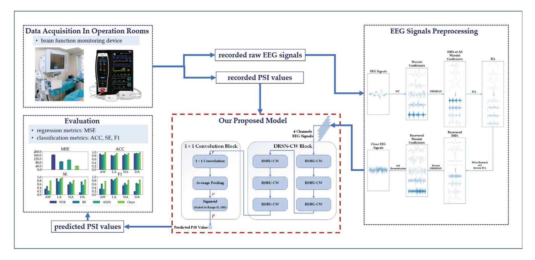
**Figure 1.** Our workflow.
## 2. Materials and Methods
### 2.1. Dataset
The dataset used in this research, which contains 18 patients aged 66–92 years old, was registered, collected, and provided by Peking University People's Hospital. During hip fracture repair surgeries, the patients received spinal anesthesia, and midazolam was given to achieve a soothing state. The raw EEG signals were recorded using the NEXT Generation SedLine® Brain Function Monitoring (Masimo, Irvine, CA, USA) device, which was recently introduced into clinical practice and displays PSI as the index of sedation depth. The SedLine EEG sensor consists of 6 electrodes: 1 reference channel (CT), 1 ground channel (CB), and 4 active EEG channels (L1, L2, R1, and R2) placed in the frontal pole. During the midazolam anesthesia, the raw EEG signals are sampled at 178.2 Hz. The dataset we used records 4 channels' raw EEG signals, PSI values, spectral edge frequency (SEF), burst suppression ratio, electromyographic (EMG) activity, and artifact percentage.
### 2.2. EEG Signals Preprocessing
Raw EEG signals recorded in operation rooms are usually contaminated by electrical noise and other physiological (not brain-related) signals (e.g., eye movements, heartbeats, and muscle activities). Therefore, it is necessary to preprocess the raw EEG signals before the subsequent analysis.
First, we split the raw EEG signals into 4 s long segments with 50% overlap for further processing.
Second, we adopted a bandpass (1–51 Hz) finite impulse response (FIR) filter to remove the electrical noise and baseline drift. Most FIR filters are linear-phase filters and don't cause a phase distortion or delay distortion of the EEG signals. However, the artifacts, especially electrooculogram artifacts (EOAs) whose magnitude is much higher than that of EEG, often have a spectral overlap with the EEG signals. Hence, it becomes a dilemma where traditional bandpass filters cannot remove EOAs while preserving the desired EEG information.
Third, to deal with the dilemma above, we propose an EOA-removing algorithm WT-CEEMDAN-ICA based on wavelet transform (WT), complete ensemble empiricalmode decomposition with adaptive noise (CEEMDAN), and independent component analysis (ICA) technologies [24–26]. As depicted in Figure 2, the WT-CEEMDAN-ICA
163
*Sensors* **2023**, *23*, 1008
consists of 6 steps: First, the WT technique is used to decompose the raw EEG signals into several wavelet coefficients. The EOAs and EEG components in the wavelet coefficients can be considered a subset of the original EOAs and EEG components. Second, the CEEMDAN technique is adopted to decompose each wavelet coefficient into several intrinsic mode functions (IMFs). Third, the IMFs of each wavelet coefficient are decomposed into multiple independent components (ICs) by using ICA. Fourth, by setting the threshold of the sample entropy of ICs, the ICs of EOAs and EEG components are separated because they are generated by different sources and are independent of each other. Then, the IMFs of the EEG components are recovered by performing the inverse transformation of ICA on the ICs of EEG components. Fifth, the wavelet coefficients are recovered by performing the inverse transformation of CEEMDAN. Finally, the EEG signals without EOAs are reconstructed by performing the inverse transformation of WT.
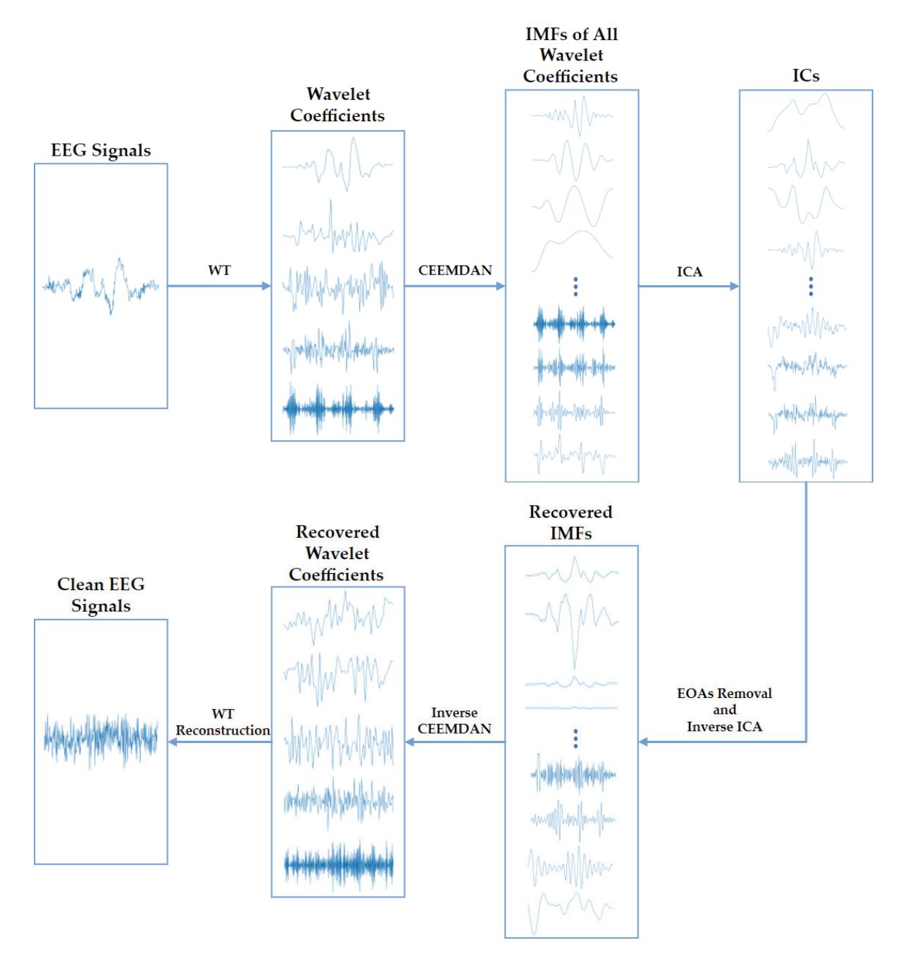
**Figure 2.** The algorithm flowchart of the WT-CEEMDAN-ICA method used to remove EOAs from EEG signals.
Finally, we combined the 4 channels of the clean EEG signals of 4 s with the corresponding PSI value as a sample. Therefore, we obtained 22,282 samples in total to evaluate the performance of our models in estimating DoA.
### 2.3. Evaluation Metrics
In this paper, we built several models to estimate DoA in terms of the predicted PSI values and evaluated their performance in terms of both regression and classification metrics. The mean squared error (MSE) was adopted to measure the difference between 164
*Sensors* **2023**, *23*, 1008
the predicted and the ground truth PSI values. In addition, we categorized patient states into 4 different anesthetized states according to the corresponding PSI values, including the awake (AW, PSI: 81–100), light anesthesia (LA, PSI: 51–80), normal anesthesia (NA, PSI: 26–50), and deep anesthesia (DA, PSI: 0–25) states. As shown in Table 1, we used the classification accuracy (ACC), sensitivity (SE), and F1-score (F1) to evaluate the models' performances on different anesthetized states.
| | Table 1. Several regression and classification evaluation metrics. | | | | | |
|--|--------------------------------------------------------------------|--|--|--|--|--|
|--|--------------------------------------------------------------------|--|--|--|--|--|
| Metric | Formula | Description |
|-----------------------------------------|-------------------------------------------------------------------|--------------------|
| MSE
(Regression) | $$$ \frac{1}{N} \times \sum_{1}^{N} (\widehat{PSI} - PSI)^{2} $$$ | Mean Squared Error |
| ACC
(Classification) | $$$ \frac{TP+TN}{TP+FP+FN+TN} $$$ | Accuracy |
| SE
(Classification) | $$$ \frac{TP}{TP+FN} $$$ | Sensitivity |
| PR
(Not used directly in this paper) | $$$ \frac{TP}{TP+FP} $$$ | Precision |
| F1
(Classification) | $$$ 2 \times \frac{SE \times PR}{SE+PR} $$$ | F1-score |
In Table 1, *N* is the number of samples, *PSI* is the predicted PSI value, *PSI* is the ground truth PSI value, *TP* is true positive and it equals the number of samples whose actual labels and predicted labels are both positive, *TN* is true negative and it equals the number of samples whose actual labels and predicted labels are both negative, *FP* is false positive and it equals the number of samples whose actual labels are negative and predicted labels are positive, and *FN* is false negative and it equals the number of samples whose actual labels are positive and predicted labels are negative.
### 2.4. Deep Learning Model
#### 2.4.1. Deep Residual Shrinkage Network
ResNets are proposed to deal with the degradation problem in deep networks [27]. ResNets introduce the shortcut connections mechanism so that the gradients are not only back-propagated layer by layer but also flow back to the beginning layers directly. As shown in Figure 3, the basic component of ResNets is a residual building block (RBB) which consists of two convolutional layers, two batch normalization (BN) layers, two rectifier linear units (ReLUs) layers, and one shortcut connection. Figure 3a is the identity block where the input feature map is the same size as the output feature map, while Figure 3b is the convolutional block where the size of the input feature map is different from that of the output feature map.
DRSN is a deep learning method that integrates soft thresholding as trainable shrinkage functions inserted into the ResNets. The DRSN forces the unimportant features to be zeros so that the extracted high-level features become more discriminative. Previous experimental results have demonstrated that the DRSN is not only capable of improving the discriminative feature learning ability but is also applicable when dealing with various signals that are disturbed by noise [28]. As depicted in Figure 4, the basic component of DRSN with channel-wise thresholds (DRSN-CW) is a residual shrinkage-building unit with channel-wise thresholds (RSBU-CW). The RSBU-CW is different from the RBB in that the RSBU-CW is distinguished by a special module for estimating thresholds used in soft thresholding. The special module mainly consists of a global-average pooling (GAP) layer, a BN layer, a ReLU layer, a sigmoid layer, and a two-layer fully connected network. The module takes the feature map *x* as its input to generate a 1D threshold vector *τ*. The values of *τ* are positive and kept in a reasonable range so that the RSBU-CW can prevent the output features from being all zero and eliminate noise-related information. The process of the module is expressed as follows:
165
*Sensors* **2023**, *23*, 1008
$$\alpha_c = \frac{1}{1 + e^{-z_c}} \tag{1}$$
$$\tau_c = \alpha_c \cdot x_{avg} \tag{2}$$
$$y_{h, w,c} = \begin{cases} x_{h,w,c} - \tau_c, & x_{h,w,c} > \tau_c \\ 0, & -\tau_c \le x_{h, w,c} \le \tau_c \\ x_{h,w,c} + \tau_c, & x_{h,w,c} < -\tau_c \end{cases}$$
$(3)$
where *h*, *w*, and *c* are the indexes of height, width, and channel of the input feature map *x*, and the output feature map *y*, respectively, *zc* is the feature at the *c*th neuron of the twolayer fully connected network, *αc* is the *c*th scaling parameter after the sigmoid layer, and *τc* is the threshold of the *c*th channel.
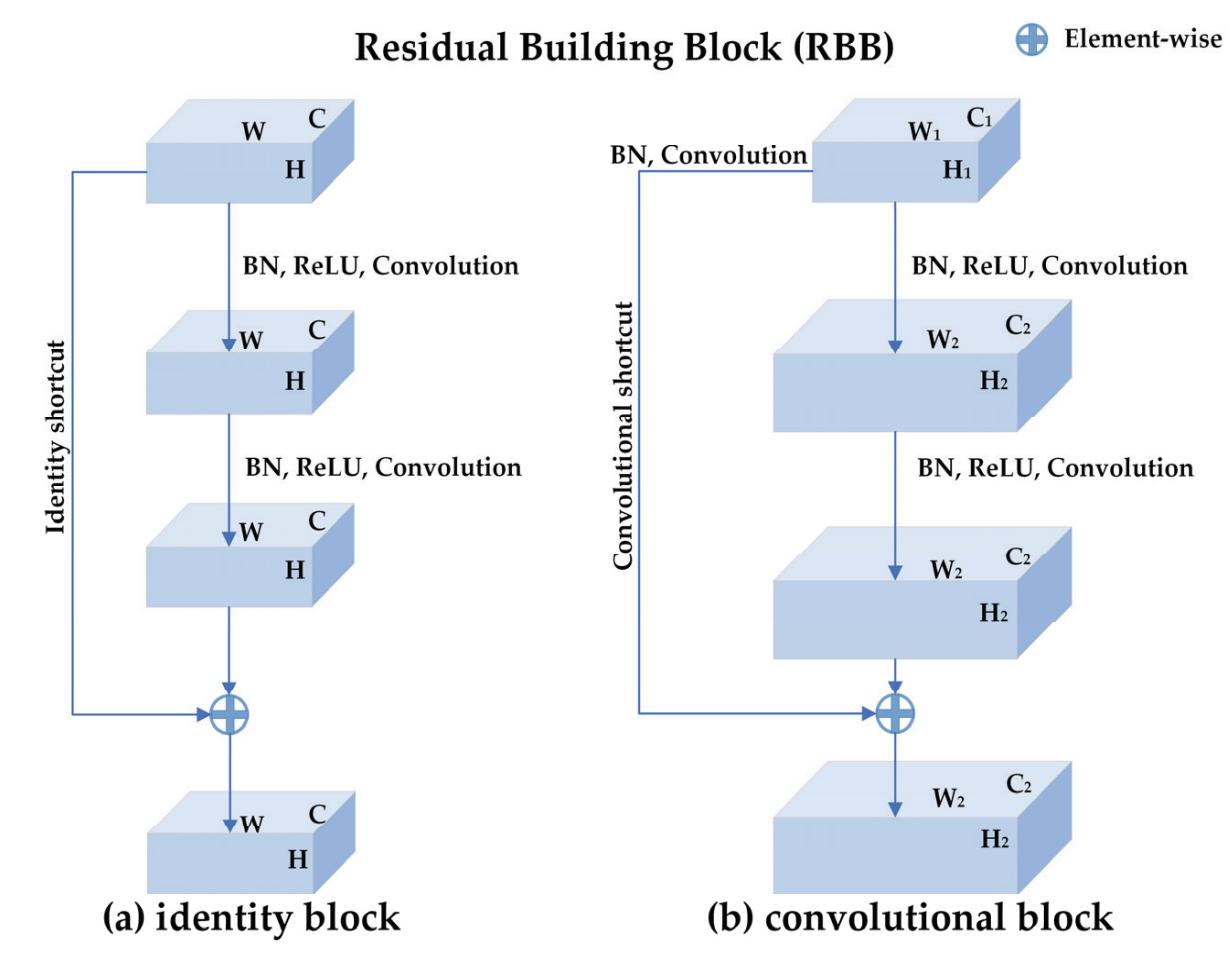
**Figure 3.** The structure of residual building block (RBB): (**a**) the identity block where the input feature map is the same size as the output feature map. H, W, and C represent the height, width, and channels of the input and output feature map, respectively. (**b**) the convolutional block where the size of the input feature map is different from that of the output feature map. There is a convolution operation and a Batch-normalization operation in the convolutional shortcut for changing the shape of the input. H1, W1, and C1 represent the height, width, and channels of the input feature map, respectively. H2, W2, and C2 represent the height, width, and channels of the output feature map, respectively. An RBB consists of two convolutional layers, two batch normalization (BN) layers, two rectifier linear units (ReLUs) layers, and one shortcut connection.
#### 2.4.2. 1 × 1 Convolution
1 × 1 convolution was proposed to increase the representation power and reduce the dimension of neural networks [29,30]. As shown in Figure 5, the size of the input feature map of the 1 × 1 convolutional layer is *H* × *W* × *C* (*H*, *W*, and *C* represent the height, width, and channels, respectively, and are henceforth represented as such in the rest of this paper), the size of the 1 × 1 convolutional kernel is 1 × 1 × *C*, and the size of the corresponding output feature map is *H* × *W* × 1. The 1 × 1 convolution does not change the height or the width of feature maps but reduces the number of channels. Therefore, a 1 × 1 convolution is effective for dimensionality reduction, adding additional non-linearity to networks, and creating smaller convolutional neural networks that retain a higher degree of accuracy.
166
*Sensors* **2023**, *23*, 1008
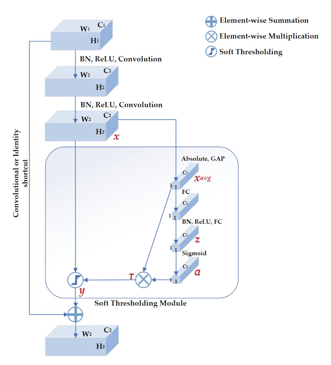
**Figure 4.** The structure of residual shrinkage building unit with channel-wise thresholds (RSBU-CW). H1, W1, and C1 represent the height, width, and channels of the input feature map, respectively. H2, W2, and C2 represent the height, width, and channels of the output feature map, respectively. There is a soft thresholding module in RSBU-CW. *xavg*, *z*, and *α* are the indicators of the feature maps used to determine the threshold *τ*. *x* and *y* are the input and output feature maps of the soft thresholding module, respectively.
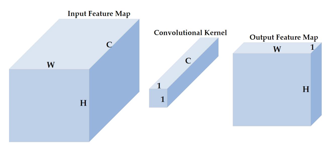
**Figure 5.** The illustration of 1 × 1 convolution. H, W, and C represent the height, width, and channels of the input feature map, respectively. A 1 × 1 convolution does not change the height or width but the number of channels of inputs.
167
*Sensors* **2023**, *23*, 1008
#### 2.4.3. Proposed Regression Model
We proposed a deep learning regression model to estimate the depth of anesthesia based on DRSN-CW and 1 × 1 convolution. The architecture of our proposed model is depicted in Figure 6. There are two blocks in the model: the DRSN-CW block and the 1 × 1 convolution block. We implemented the RSBU-CW with 1D convolutions because the input EEG signals of each channel are 1D time series. Besides this, we replaced the activation function ReLU in the RSBU-CW with the exponential linear unit (ELU) for better performance. The DRSN-CW block was used to automatically extract high-level feature representations from the EEG signals. In general, fully connected networks are adopted to predict the desired values using the final representations. However, the parameters of a fully connected network are usually more than half of those of the whole model, resulting in the risk of overfitting and expensive computation. Therefore, we used the 1 × 1 convolution instead of the fully connected network to predict the PSI values. The size of the final representation *r* was 1 × *W* × 16, and the 1D convolution layer reduced the dimension of *r* into 1 × *W* × 1. Then, an average pooling layer was used to generate a single value *v*. Finally, the predicted PSI value *p* was generated with a Sigmoid function and scaled to the range of (0, 100) as follows:
$$p = \frac{100}{1 + e^{-v}},\tag{4}$$
and we used MSE as the loss function of our proposed regression model.
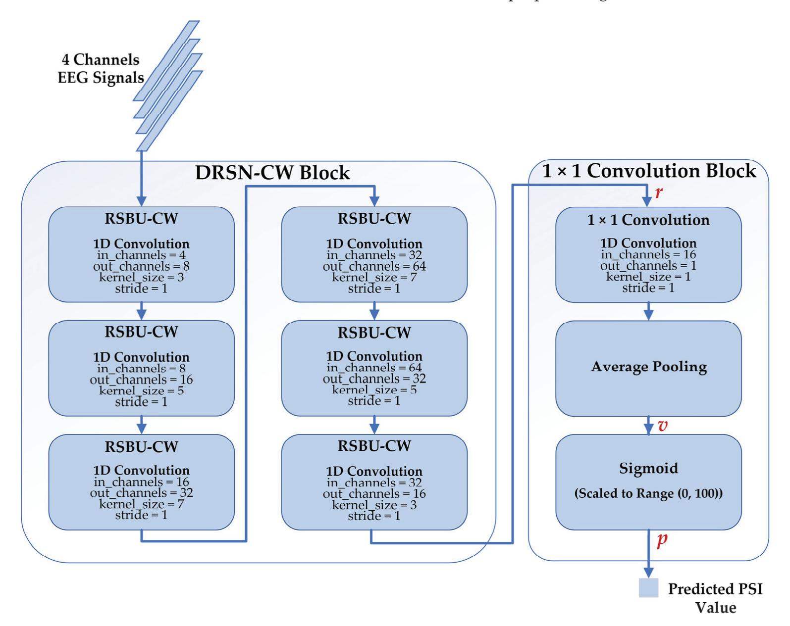
**Figure 6.** The structure of our proposed model consists of the DRSN-CW block and 1 × 1 convolution block. The inputs of our proposed model are 4 channel-EEG signals, and the outputs are the corresponding predicted PSI values.
168
*Sensors* **2023**, *23*, 1008
### 2.5. Conventional Models
#### 2.5.1. Features Extraction
The conventional models usually use extracted features instead of the clean EEG signals as inputs. Therefore, we extracted several features relating to PSI from the EEG samples according to what Drover et al. [12] propose.
#### • Band Power
The recorded EEG signals consist of 4 different channels (FP1, FP2, F7, and F8, according to the international 10–20 system [31]). We computed the power spectral density for each frequency band with the MNE-Python package [32]. The EEG signals can be divided into five frequency bands (δ [1–4 Hz], θ [4–8 Hz], α [8–14 Hz], β [14–31 Hz], and γ [31–51 Hz]) according to their frequency ranges. Then, we computed the band powers of each frequency band using the multitaper spectral-analysis method [33]. Furthermore, the relative band power of a specific-frequency band could be calculated by dividing it by the total band power.
#### • Spectral Edge Frequency
The spectral edge frequency (SEF) is a popular measure used in EEG monitoring [34]. SEF95 is the frequency below which 95% of the total power of a given signal is located. We computed the SEF95 in the left and right hemispheres, respectively.
#### • Sample Entropy
Approximate entropy is a measure describing the complexity and regularity of time series, while sample entropy is a similar but more accurate method to approximate entropy [35,36]. Sample entropy has been used to estimate DoA and has achieved good results [16]. Based on the existing research's parameter settings, we calculated each channel's sample entropy values as the last 4 features.
In total, we extracted 14 features from the EEG signals, including the total power in the frontopolar region, the total power in the left hemisphere, the total power in the right hemisphere, the band power changes in δ, the band power changes in θ, the band power changes in α, the band power changes in β, the band power changes in γ, the SEF95 in the left hemisphere, the SEF95 in the right hemisphere, and the sample entropy values of 4 channels, respectively.
### 2.5.2. Conventional Regression Models
This paper used three conventional regression models to estimate DoA as comparisons, including the support vector regression (SVR), random forest (RF), and ANN.
#### • Support Vector Machine
SVM is a classic supervised machine learning model that analyzes data for both classification and regression tasks [37], and the model for regression tasks is support vector regression (SVR) [38]. Although there are slight differences between SVR and SVM, they share the same core idea of finding a hyperplane that best divides the training samples. In this paper, we used SVR with radial basis function kernel.
#### • Random Forest
RF is a classic supervised learning algorithm that uses an ensemble learning method for classification and regression tasks. RF operates by constructing multiple decision trees and outputting the mean prediction of the individual trees. In this paper, we used 300 trees to train the model.
#### • Artificial Neural Network
ANN is a computing system inspired by the biological neural networks that constitute animal brains [39]. ANN is a nonlinear statistical model that learns complex relationships between inputs and outputs to find new patterns. In this paper, we implemented an ANN of the structure 14–64–16–1 to predict the PSI values.
169
*Sensors* **2023**, *23*, 1008
## 3. Results
### 3.1. Experimental Settings
In this section, we describe the experimental settings in detail. To evaluate the performances of different models, we conducted a five-fold cross-validation: First, we shuffled the whole dataset randomly and split the dataset into five groups. Second, for each group, we took the dataset as the test set, trained models on the other 4 groups, and evaluated models on the test set. Finally, we summarized the results of the five-fold cross-validation with the mean and variance of all metrics. Besides this, we also implemented a cross-subject validation as a supplement. Figure 7 illustrates the distribution of the dataset used in this study. The numbers of samples of different anesthetized states are unbalanced: 49.14% of samples belong to AW, while only 3.31% of samples belong to DA.
**Figure 7.** The data distribution of the dataset used in this study.
Each EEG sample contains 4 channels of 4 s EEG signals whose dimension is 4 × 712. The amplitudes and variances of EEG signals among different individuals and situations could vary greatly. Therefore, the data standardization was adopted to make our proposed model converge faster and generalize better: First, we transformed the EEG signals of the train and test sets into a 1D vector that has 2848 columns. Second, we computed each column's mean and standard deviation on the train set. Third, we standardized each column by subtracting its mean and dividing it by its standard deviation on both the train and test sets. Finally, we reshaped the 1D vectors into EEG signals whose dimension is 4 × 712. A similar data standardization was applied to the samples containing 14 extracted features for the conventional feature-based models.
We implemented our proposed model and the ANN model with PyTorch [40]. The Adam optimization was applied to minimize the MSE loss function. We set the batch size as 64, the initial learning rate as 0.005, and the maximum of epochs as 256. The learning rate decreased by 10% every 20 epochs, and we used L2 normalization to prevent overfitting. We implemented the SVR and RF models with Scikit-learn [41].
### 3.2. Experimental Results
We compared our proposed model with three conventional models. As shown in Table 2, our proposed model has good regression performance and classification ability. In the MSE metric, the mean and STD of our proposed model are significantly less than the conventional models, indicating our proposed model's impressive regression and generalization performance. Our proposed model yields the highest ACC, SE, and F1 in the classification metrics, especially the ACC and SE values (ACC: 0.9503, SE: 0.8411) in comparison with conventional models (ACC ≤ 0.8640, SE ≤ 0.6685). Moreover, as depicted
170
*Sensors* **2023**, *23*, 1008
in Figure 8, our proposed model exhibits the most balanced performance for different anesthetized states.
**Table 2.** The regression and classification results (mean ± STD) of our proposed model and three conventional models. The mean squared error (MSE) result is the average of the five-fold crossvalidation where we split all the samples into five groups, four groups are used as the train set, and one group is used as the test set for each cross-validation. The accuracy (ACC), sensitivity (SE), and F1-score (F1) results are the macro-averaging (we compute the metrics independently for each anesthetized state and then take the average) results of the 4 different anesthetized states.
| Metrics | SVR | RF | ANN | Our Proposed Model |
|---------|-----------------|-----------------|-----------------|--------------------|
| MSE | 166.02 ± 7.77 | 90.95 ± 4.88 | 109.20 ± 5.80 | 40.35 ± 3.22 |
| ACC | 0.8596 ± 0.0574 | 0.8640 ± 0.0720 | 0.8606 ± 0.0380 | 0.9503 ± 0.0224 |
| SE | 0.4825 ± 0.3391 | 0.6685 ± 0.1266 | 0.5650 ± 0.2801 | 0.8411 ± 0.0790 |
| F1 | 0.475 ± 0.2941 | 0.6770 ± 0.0840 | 0.5901 ± 0.2337 | 0.8395 ± 0.0812 |
**Figure 8.** The classification performances (ACC, SE, and F1) of all the models on different anesthetized states (AW, LA, NA, and DA) and the regression performance (MSE) of all the models.
We illustrate one of the five-fold cross-validation results in Figure 9. There is a relatively high similarity between the ground truth PSI values and the predicted PSI values of our proposed model, and the Spearman's rank correlation coefficient is 0.9344.
To demonstrate the effectiveness of the soft thresholding module in the RSBU-CW, we conducted an ablation experiment. We evaluated our proposed model's regression and classification performances with and without the soft thresholding module in the RSBU-CW. As shown in Figure 10, when the soft thresholding module is ablated, the MSE increases by 38.33, and the classification performances significantly decline as well.
In addition, to further illustrate the effectiveness and robustness of the model we proposed, we conducted a 5-fold cross-validation, which is cross-subject. First, we divided all the subjects into five groups. Specifically, there are four subjects (4122 samples in total) in Group A, four (4271 samples in total) in Group B, four (4590 samples in total) in Group C, three (4793 samples in total) in Group D, and three (5056 samples in total) in Group E.
Similarly, for each group separately, we took it as the test set, trained models on the other four groups, and evaluated models on the test set. Finally, we summarized the results of the five-fold cross-validation with the mean and variance of all metrics. The results are shown in Table 3 and Figure 11. As can be seen, our proposed model still achieves a better performance in both regression and classification. More precisely, even for the best-performing random forest among the three conventional models, its mean square error is much higher than ours.
171
*Sensors* **2023**, *23*, 1008
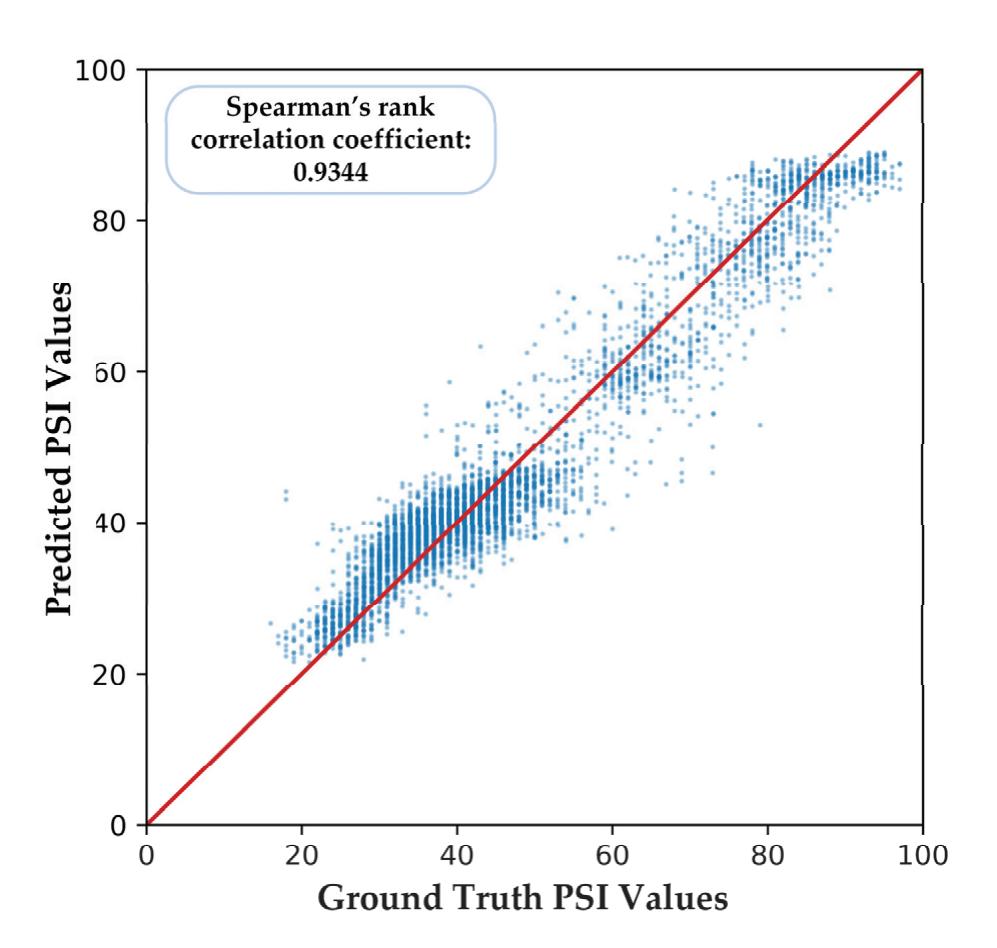
**Figure 9.** Part of the predicted PSI values of our proposed model. The red line represents the ideal prediction model where the predicted PSI values equal the ground truth PSI values exactly.
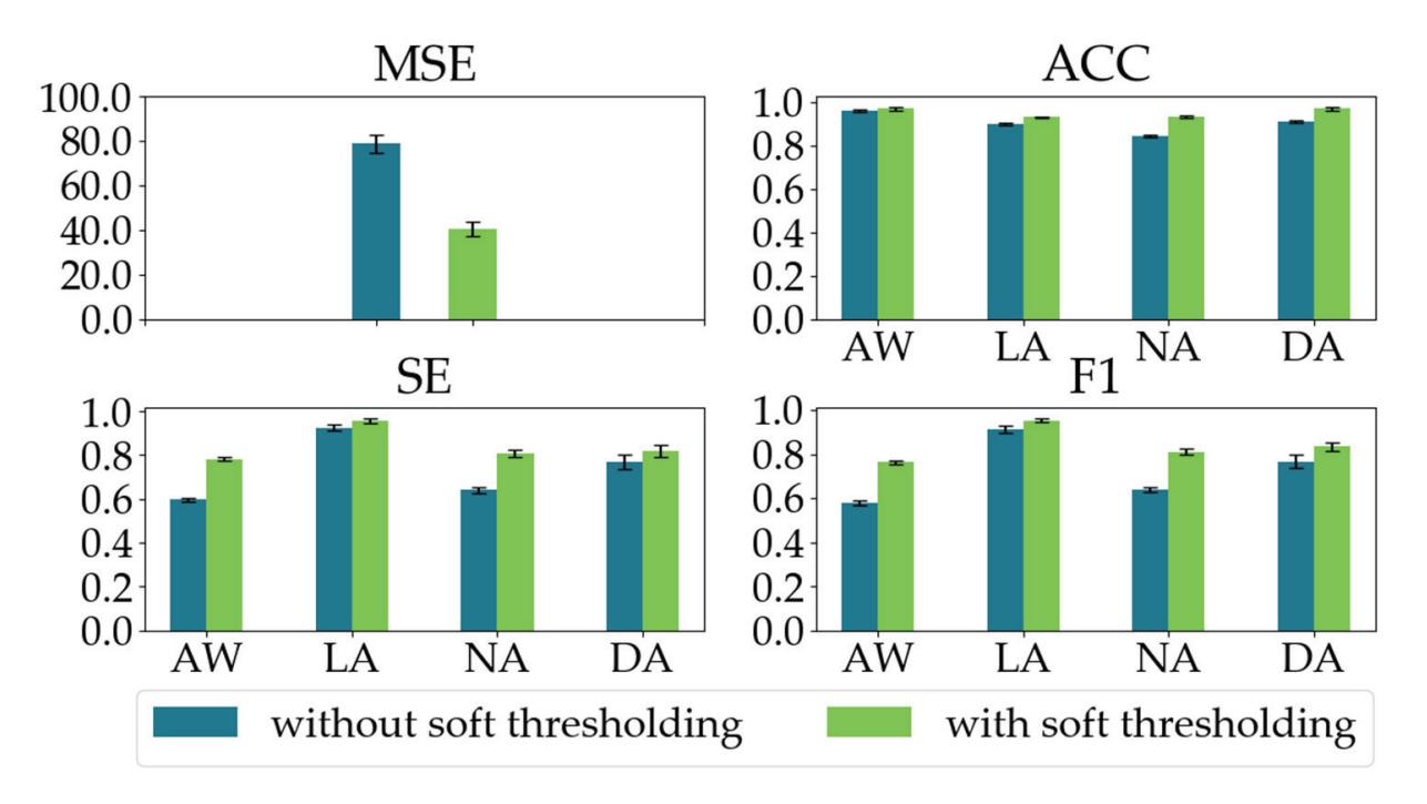
**Figure 10.** The regression and classification performances of the two models in the ablation experiment on the soft thresholding module in the RSBU-CW.
**Table 3.** The regression and classification results (mean ± STD) of our proposed model and three conventional models in cross-subject validation.
| Metrics | SVR | RF | ANN | Our Proposed Model |
|---------|-----------------|-----------------|-----------------|--------------------|
| MSE | 173.22 ± 8.56 | 97.56 ± 6.88 | 133.49 ± 5.40 | 49.22 ± 4.62 |
| ACC | 0.7908 ± 0.1187 | 0.8420 ± 0.0765 | 0.8216 ± 0947 | 0.9203 ± 0.0470 |
| SE | 0.4675 ± 0.3391 | 0.6575 ± 0.1266 | 0.5700 ± 0.1414 | 0.8054 ± 0.0243 |
| F1 | 0.4599 ± 0.2132 | 0.6670 ± 0.0821 | 0.5852 ± 0.1274 | 0.8070 ± 0.0306 |
172
*Sensors* **2023**, *23*, 1008
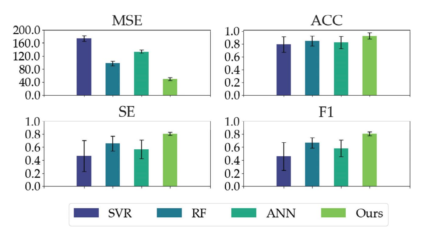
**Figure 11.** The classification performances (ACC, SE, and F1) of all the models on different anesthetized states (AW, LA, NA, and DA) and the regression performance (MSE) of all the models in cross-subject validation.
Similarly, we computed Figure 12 to show the correlation between predicted PSI values and ground truth, and Spearman's rank correlation coefficient is 0.9172, which is still significant.
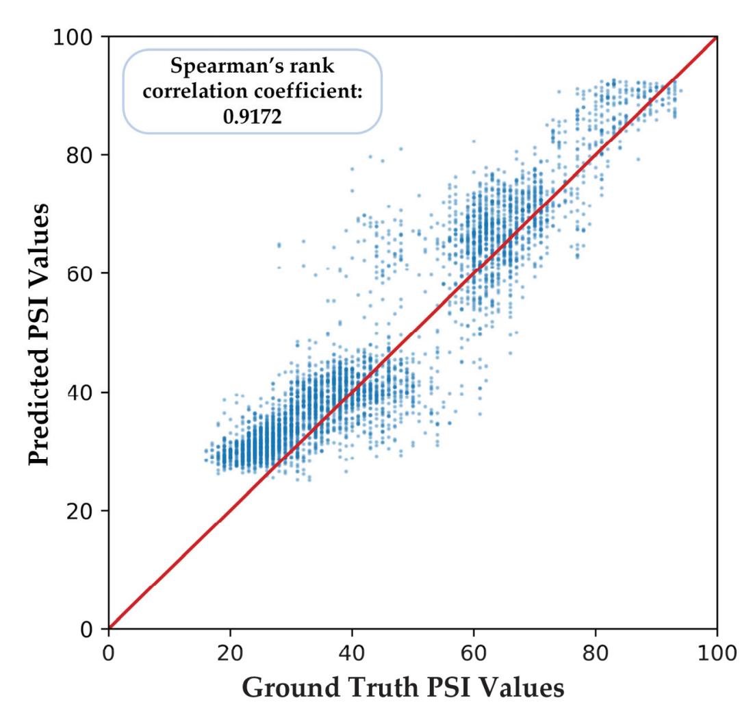
**Figure 12.** Part of the predicted PSI values of our proposed model in cross-subject validation.
## 4. Discussion
In previous studies, most researchers used the EEG-based features with conventional models (e.g., ANN, RF, SVR) to estimate DoA in terms of BIS values. However, the regression and classification performances could have been more satisfactory. Besides, the performances of different anesthetized states needed to be more balanced. Thanks to the 173
*Sensors* **2023**, *23*, 1008
development of deep learning methods, some researchers adopted deep learning models to process EEG signals directly to assess DoA. The results of deep learning models were better than that of conventional models. These conventional machine-learning methods are based on various features extracted manually [42]. In comparison, the highlight of our proposed model, which mainly consists of the DRSN-CW and the 1 × 1 convolution networks, is that the model can automatically extract features in the training process. Therefore, the trouble and difficulty of manually extracting features are resolved.
The actual experimental results also demonstrate the superiority of our proposed model over other traditional methods. Furthermore, our proposed model achieves the most balanced results for different anesthetized states among all the models, especially for DA, even though there is a dilemma of limited subjects. In addition, we conducted an ablation experiment to demonstrate the effectiveness of the soft thresholding module for EEG-signal processing. Therefore, our proposed model is a promising and feasible method for estimating DoA.
There are several noteworthy points of this research:
- 1. The recorded raw EEG signals are usually contaminated by electrical noise and other physiological signals. We used bandpass finite filters to remove electrical noise, and the WT-CEEMDAN-ICA algorithm to extract clean EEG signals.
- 2. We adopted deep learning models to extract discriminative features automatically instead of extracting features manually from EEG signals.
- 3. To improve our proposed model's generalization ability and convergence speed, we standardized the EEG signals.
- 4. DRSN-CW can deal with signals disturbed by noise, which is suitable for EEG-signal processing.
The 1 × 1 convolution network has much fewer parameters than a fully connected network, decreasing the overfitting risk while retaining better performance. Our proposed deep learning model is capable of mimicking PSI values and distinguishing different anesthetized states by directly processing EEG signals, indicating that deep learning methods have tremendous advantage over conventional methods in processing EEG signals to estimate DoA. This research provides inspiration to develop an accurate and reliable DoA assessment system beyond the proprietary PSI or BIS algorithm. Although we used PSI values as DoA labels in this study, our proposed model is not limited to mimicking PSI values. By combining PSI or BIS values with expert assessments of anesthetized levels and building a large-scale DoA dataset, deep learning methods could be evaluated and improved from a more comprehensive perspective. Therefore, directly processing EEG signals with deep learning models is a promising and feasible method to estimate DoA.
## 5. Conclusions
Reliable DoA monitoring is essential for surgeries. For this purpose, we utilized an effective preprocess for noise filtering and propose a deep learning model, mainly consisting of the DRSN-CW and 1 × 1 convolution networks, to estimate DoA in terms of PSI values. We also compared our proposed model with three conventional feature-based models on the dataset of 18 patients. The experimental results show that our proposed model remarkably surpasses conventional models in regression and classification performances. The results of the ablation study and cross-subject validation further illustrate the robustness and structural advantages of the model. Deep learning models are promising and feasible to assess DoA during surgery.
At the same time, we also realize that the information contained in a single kind of physiological signal is limited, which determines the upper limit of the performance of our proposed model. Therefore, to develop a more accurate and reliable DoA assessment system in the future, we will include more signals (such as ECG, EMG, blood pressure, etc.) besides EEG. We will build a larger DoA dataset that combines the PSI values and expert assessments of anesthetized levels as DoA labels, thereby improving our proposed deep learning model.
174
*Sensors* **2023**, *23*, 1008
**Author Contributions:** Conceptualization, M.S., Q.R. and H.Z.; methodology, M.S., Z.H., G.X. and Q.R.; software, M.S., G.X. and B.X.; validation, Z.H. and G.X.; investigation, Z.H. and B.X.; data curation, Z.H. and H.Z.; visualization, M.S., G.X. and B.X.; writing—original draft preparation, M.S., Z.H., G.X. and Q.R.; writing—review and editing, M.S., Z.H., H.Z. and Q.R.; project administration, Q.R. and H.Z.; funding acquisition, Q.R. and H.Z. All authors have read and agreed to the published version of the manuscript.
**Funding:** This work was supported in part by Beijing Municipal Natural Science Foundation (grant No. M22010), the Ministry of Science and Technology of the People's Republic of China with Funding No. 2020AAA0109600 (funding recipient, Xiuyuan Chen, M.D. Department of Throacic Surgery, Peking University People's Hospital) and Project (RDY 2019-17) from Peking University People's Hospital Scientific Research Development Funds, Beijing, China.
**Institutional Review Board Statement:** The study was conducted in accordance with the Declaration of Helsinki, and approved by the Institutional Review Board of Peking University People's Hospital on 28 November 2019 (protocol code 2019PHB164-01).
**Informed Consent Statement:** Informed consent was obtained from all subjects involved in the study.
**Data Availability Statement:** The code of our proposed model will be available after acceptance, and the dataset of this study is available from the corresponding author upon reasonable request.
**Acknowledgments:** The work was supported in part by High-performance Computing Platform of Peking University. The study sponsors had no involvements in the study design, nor in the collection, analysis, and interpretation of data; in the writing of the manuscript; and in the decision to submit the manuscript for publication.
**Conflicts of Interest:** The authors declare no conflict of interest.
### References
- 1. Hajat, Z.; Ahmad, N.; Andrzejowski, J. The role and limitations of EEG-based depth of anaesthesia monitoring in theatres and intensive care. *Anaesthesia* **2017**, *72*, 38–47. [CrossRef] [PubMed]
- 2. Kent, C.; Domino, K.B. Depth of anesthesia. *Curr. Opin. Anaesthesiol.* **2009**, *22*, 782–787. [CrossRef] [PubMed]
- 3. Fahy, B.G.; Chau, D.F. The technology of processed electroencephalogram monitoring devices for assessment of depth of anesthesia. *Anesth. Analg.* **2018**, *126*, 111–117. [CrossRef] [PubMed]
- 4. Aydemir, E.; Tuncer, T.; Dogan, S.; Gururajan, R.; Acharya, U.R. Automated major depressive disorder detection using melamine pattern with EEG signals. *Appl. Intell.* **2021**, *51*, 6449–6466. [CrossRef]
- 5. Loh, H.W.; Ooi, C.P.; Aydemir, E.; Tuncer, T.; Dogan, S.; Acharya, U.R. Decision support system for major depression detection using spectrogram and convolution neural network with EEG signals. *Expert Syst.* **2022**, *39*, e12773. [CrossRef]
- 6. Tasci, G.; Loh, H.W.; Barua, P.D.; Baygin, M.; Tasci, B.; Dogan, S.; Acharya, U.R. Automated accurate detection of depression using twin Pascal's triangles lattice pattern with EEG Signals. *Knowl.-Based Syst.* **2022**, *260*, 110190. [CrossRef]
- 7. Xiao, G.; Shi, M.; Ye, M.; Xu, B.; Chen, Z.; Ren, Q. 4D attention-based neural network for EEG emotion recognition. *Cogn. Neurodynamics.* **2022**, *16*, 805–818. [CrossRef]
- 8. Liang, Z.; Wang, Y.; Sun, X.; Li, D.; Voss, L.J.; Sleigh, J.W.; Li, X. EEG entropy measures in anesthesia. *Front. Comput. Neurosci.* **2015**, *9*, 16. [CrossRef]
- 9. Saadeh, W.; Khan, F.H.; Altaf, M.A.B. Design and implementation of a machine learning based EEG processor for accurate estimation of depth of anesthesia. *IEEE Trans. Biomed. Circuits Syst.* **2019**, *13*, 658–669. [CrossRef]
- 10. Khan, F.H.; Ashraf, U.; Altaf, M.A.B.; Saadeh, W. A patient-specific machine learning based EEG processor for accurate estimation of depth of anesthesia. In Proceedings of the 2018 IEEE Biomedical Circuits and Systems Conference (BioCAS), Cleveland, OH, USA, 17–19 October 2018; pp. 1–4.
- 11. Gonsowski, C.T. Anesthesia Awareness and the Bispectral Index. *N. Engl. J. Med.* **2008**, *359*, 427–431.
- 12. Drover, D.; Ortega, H.R. Patient state index. *Best Pract. Res. Clin. Anaesthesiol.* **2006**, *20*, 121–128. [CrossRef]
- 13. Ji, S.H.; Jang, Y.E.; Kim, E.H.; Lee, J.H.; Kim, J.T.; Kim, H.S. Comparison of Bispectral Index and Patient State Index during Sevoflurane Anesthesia in Children: A Prospective Observational Study. Available online: https://www.researchgate. net/publication/343754479\_Comparison\_of\_bispectral\_index\_and\_patient\_state\_index\_during\_sevoflurane\_anesthesia\_in\_ children\_a\_prospective\_observational\_study (accessed on 3 November 2020).
- 14. Li, P.; Karmakar, C.; Yearwood, J.; Venkatesh, S.; Palaniswami, M.; Liu, C. Detection of epileptic seizure based on entropy analysis of short-term EEG. *PLoS ONE* **2018**, *13*, e0193691. [CrossRef] [PubMed]
- 15. Olofsen, E.; Sleigh, J.W.; Dahan, A. Permutation entropy of the electroencephalogram: A measure of anaesthetic drug effect. *BJA Br. J. Anaesth.* **2008**, *101*, 810–821. [CrossRef] [PubMed]
- 16. Liu, Q.; Ma, L.; Fan, S.Z.; Abbod, M.F.; Shieh, J.S. Sample entropy analysis for the estimating depth of anaesthesia through human EEG signal at different levels of unconsciousness during surgeries. *PeerJ* **2018**, *6*, e4817. [CrossRef]
175
*Sensors* **2023**, *23*, 1008
- 17. Esmaeilpour, M.; Mohammadi, A. Analyzing the EEG signals in order to estimate the depth of anesthesia using wavelet and fuzzy neural networks. *Int. J. Interact. Multimed. Artif. Intell.* **2016**, *4*, 12. [CrossRef]
- 18. Ortolani, O.; Conti, A.; Di Filippo, A.; Adembri, C.; Moraldi, E.; Evangelisti, A.; Roberts, S.J. EEG signal processing in anaesthesia. Use of a neural network technique for monitoring depth of anaesthesia. *Br. J. Anaesth.* **2002**, *88*, 644–648. [CrossRef] [PubMed]
- 19. Shalbaf, A.; Saffar, M.; Sleigh, J.W.; Shalbaf, R. Monitoring the depth of anesthesia using a new adaptive neurofuzzy system. *IEEE J. Biomed. Health Inform.* **2017**, *22*, 671–677. [CrossRef]
- 20. Gu, Y.; Liang, Z.; Hagihira, S. Use of Multiple EEG Features and Artificial Neural Network to Monitor the Depth of Anesthesia. *Sensors* **2019**, *19*, 2499. [CrossRef]
- 21. Esteva, A.; Robicquet, A.; Ramsundar, B.; Kuleshov, V.; DePristo, M.; Chou, K.; Dean, J. A guide to deep learning in healthcare. *Nat. Med.* **2019**, *25*, 24–29. [CrossRef]
- 22. Lee, H.C.; Ryu, H.G.; Chung, E.J.; Jung, C.W. Prediction of bispectral index during target-controlled infusion of propofol and remifentanil: A deep learning approach. *Anesthesiology* **2018**, *128*, 492–501. [CrossRef]
- 23. Afshar, S.; Boostani, R. A Two-stage deep learning scheme to estimate depth of anesthesia from EEG signals. In Proceedings of the 2020 27th National and 5th International Iranian Conference on Biomedical Engineering (ICBME), Tehran, India, 26–27 November 2020.
- 24. Castellanos, N.P.; Makarov, V.A. Recovering EEG brain signals: Artifact suppression with wavelet enhanced independent component analysis. *J. Neurosci. Methods* **2006**, *158*, 300. [CrossRef] [PubMed]
- 25. Mammone, N.; La Foresta, F.; Morabito, F.C. Automatic artifact rejection from multichannel scalp EEG by Wavelet ICA. *IEEE Sens. J.* **2012**, *12*, 533–542. [CrossRef]
- 26. Torres, M.E.; Colominas, M.A.; Schlotthauer, G.; Flandrin, P. A complete ensemble empirical mode decomposition with adaptive noise. In Proceedings of the 2011 IEEE International Conference on Acoustics, Speech and Signal Processing (ICASSP), Prague, Czech Republic, 22–27 May 2011.
- 27. He, K.; Zhang, X.; Ren, S.; Sun, J. Deep residual learning for image recognition. In Proceedings of the IEEE Conference on Computer Vision and Pattern Recognition (CVPR), Las Vegas, NV, USA, 27–30 June 2016.
- 28. Zhao, M.; Zhong, S.; Fu, X.; Tang, B.; Pecht, M. Deep residual shrinkage networks for fault diagnosis. *IEEE Trans. Ind. Inform.* **2019**, *16*, 4681–4690. [CrossRef]
- 29. Lin, M.; Chen, Q.; Yan, S. Network in network. *arXiv* **2013**, arXiv:1312.4400.
- 30. Szegedy, C.; Liu, W.; Jia, Y.; Sermanet, P.; Reed, S.; Anguelov, D.; Rabinovich, A. Going deeper with convolutions. In Proceedings of the IEEE Conference on Computer Vision and Pattern Recognition, Boston, MA, USA, 7–12 June 2015; pp. 1–9.
- 31. Seeck, M.; Koessler, L.; Bast, T.; Leijten, F.; Michel, C.; Baumgartner, C.; Beniczky, S. The standardized EEG electrode array of the IFCN. *Clin. Neurophysiol.* **2017**, *128*, 2070–2077. [CrossRef]
- 32. Alexandre, G. MEG and EEG data analysis with MNE-Python. *Front. Neurosci.* **2013**, *7*, 267.
- 33. Prerau, M.J.; Brown, R.E.; Bianchi, M.T.; Ellenbogen, J.M.; Purdon, P.L. Sleep neurophysiological dynamics through the lens of multitaper spectral analysis. *Physiology* **2017**, *32*, 60–92. [CrossRef]
- 34. Obert, D.P.; Schweizer, C.; Zinn, S.; Kratzer, S.; Hight, D.; Sleigh, J.; Kreuzer, M. The influence of age on EEG-based anaesthesia indices. *J. Clin. Anesth.* **2021**, *73*, 110325. [CrossRef]
- 35. Pincus, S.M. Approximate entropy as a measure of system complexity. *Proc. Natl. Acad. Sci. USA* **1991**, *88*, 2297–2301. [CrossRef]
- 36. Richman, J.S.; Lake, D.E.; Moorman, J.R. Sample Entropy. In *Methods in Enzymology*; Elsevier: Amsterdam, The Netherlands, 2004; pp. 172–184.
- 37. Vapnik, V. *The Nature of Statistical Learning Theory*; Springer Science & Business Media: Berlin/Heidelberg, Germany, 2013.
- 38. Rodriguez-Perez, R.; Vogt, M.; Bajorath, J. Support vector machine classification and regression prioritize different structural features for binary compound activity and potency value prediction. *ACS omega* **2017**, *2*, 6371–6379. [CrossRef]
- 39. Shahid, N.; Rappon, T.; Berta, W. Applications of artificial neural networks in health care organizational decision-making: A scoping review. *PloS ONE* **2019**, *14*, e0212356. [CrossRef]
- 40. Paszke, A.; Gross, S.; Massa, F.; Lerer, A.; Bradbury, J.; Chanan, G.; Chintala, S. PyTorch: An imperative style, high-performance deep learning library. *Adv. Neural Inf. Process Syst.* **2019**, *32*, 8026–8037.
- 41. Pedregosa, F.; Varoquaux, G.; Gramfort, A.; Michel, V.; Thirion, B.; Grisel, O.; Duchesnay, É. Scikit-learn: Machine Learning in Python. *J. Mach. Learn. Res.* **2011**, *12*, 2825–2830.
- 42. Acharya, U.R.; Oh, S.L.; Hagiwara, Y.; Tan, J.H.; Adeli, H.; Subha, D.P. Automated EEG-based screening of depression using deep convolutional neural network. *Comput. Methods Programs Biomed.* **2018**, *161*, 103–113. [CrossRef]
**Disclaimer/Publisher's Note:** The statements, opinions and data contained in all publications are solely those of the individual author(s) and contributor(s) and not of MDPI and/or the editor(s). MDPI and/or the editor(s) disclaim responsibility for any injury to people or property resulting from any ideas, methods, instructions or products referred to in the content.
176


*Article*
# An Efficient Machine Learning-Based Emotional Valence Recognition Approach Towards Wearable EEG
**Lamiaa Abdel-Hamid**
Department of Electronics & Communication, Faculty of Engineering, Misr International University (MIU), Heliopolis, Cairo P.O. Box 1, Egypt; lamiaa.a.hamid@miuegypt.edu.eg
**Abstract:** Emotion artificial intelligence (AI) is being increasingly adopted in several industries such as healthcare and education. Facial expressions and tone of speech have been previously considered for emotion recognition, yet they have the drawback of being easily manipulated by subjects to mask their true emotions. Electroencephalography (EEG) has emerged as a reliable and cost-effective method to detect true human emotions. Recently, huge research effort has been put to develop efficient wearable EEG devices to be used by consumers in out of the lab scenarios. In this work, a subject-dependent emotional valence recognition method is implemented that is intended for utilization in emotion AI applications. Time and frequency features were computed from a single time series derived from the Fp1 and Fp2 channels. Several analyses were performed on the strongest valence emotions to determine the most relevant features, frequency bands, and EEG timeslots using the benchmark DEAP dataset. Binary classification experiments resulted in an accuracy of 97.42% using the alpha band, by that outperforming several approaches from literature by ~3–22%. Multiclass classification gave an accuracy of 95.0%. Feature computation and classification required less than 0.1 s. The proposed method thus has the advantage of reduced computational complexity as, unlike most methods in the literature, only two EEG channels were considered. In addition, minimal features concluded from the thorough analyses conducted in this study were used to achieve state-of-the-art performance. The implemented EEG emotion recognition method thus has the merits of being reliable and easily reproducible, making it well-suited for wearable EEG devices.
**Keywords:** classification; EEG; emotion recognition; prefrontal channels; time and frequency features
**Citation:** Abdel-Hamid, L. An Efficient Machine Learning-Based Emotional Valence Recognition Approach Towards Wearable EEG. *Sensors* **2023**, *23*, 1255. https:// doi.org/10.3390/s23031255
Academic Editors: Yifan Zhao, Yuzhu Guo and Fei He
Received: 3 December 2022 Revised: 14 January 2023 Accepted: 17 January 2023 Published: 21 January 2023

**Copyright:** © 2023 by the author. Licensee MDPI, Basel, Switzerland. This article is an open access article distributed under the terms and conditions of the Creative Commons Attribution (CC BY) license (https:// creativecommons.org/licenses/by/ 4.0/).
## 1. Introduction
Emotion artificial intelligence (AI), also known as affective computing, is the study of systems that can recognize, process, and respond to the different human emotions, thereby making people's lives more convenient [1]. Emotion AI is an interdisciplinary field that combines artificial intelligence, cognitive science, psychology, and neuroscience. In 2019, the emotion AI industry was worth about 21.6 billion dollars, and its value was predicted to reach 56 billion dollars by the year 2024 [2].
Emotions are mental states created in response to events occurring to us or in the world around us. A large body of research since the 1970s showed that basic emotions, such as happiness, sadness, and anger are similarly expressed among different cultures [3]. James Russell, a renowned American psychologist, suggested a dimensional approach in which all human emotions could be expressed in terms of valence and arousal [4]. Valence refers to the extent to which an emotion is pleasant (positive/happy) or unpleasant (negative/sad), whereas arousal (intensity) refers to the strength or mildness of a given emotion (Figure 1). Russell's valence-arousal model is very popular owing to its simplicity and efficacy, both which lead to it being widely adopted in emotion AI systems [5].
*Sensors* **2023**, *23*, 1255. https://doi.org/10.3390/s23031255 https://www.mdpi.com/journal/sensors
177
*Sensors* **2023**, *23*, 1255
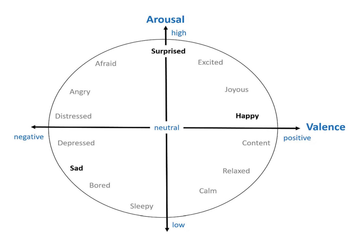
**Figure 1.** Valence-arousal model [6].
Emotions can be detected from a person's facial expressions and tone of speech. Although these methods were previously considered for automatic emotion recognition [7,8], they both have the limitation of being easily manipulated by a person to hide his/her true emotions [5,9]. Electroencephalography (EEG) is a non-invasive technique that can measure spontaneous human brain activity while providing excellent temporal resolution yet limited spatial resolution [10]. EEG can thus provide a reliable method to detect and monitor true, unmanipulated human emotions. EEG-based emotion recognition has been successfully implemented in various applications including (1) education: to measure student engagement, (2) health: to diagnosis psychological diseases, and (3) emotion-based music players: to provide a more engaging experience [11].
The cerebral cortex is the outermost layer of the brain that is associated with the highest mental capabilities. The cerebral cortex is traditionally divided into four main lobes which are the frontal (F), parietal (P), occipital (O), and temporal (T) (Figure 2). Each brain lobe is typically associated with certain functions, yet many activities require the coordination of multiple lobes [12]. The frontal lobe is responsible for cognitive functions such as emotions, memory, decision making, and problem solving, as well as voluntary movement control. The parietal lobe process information received from the outside world such as that related to touch, taste, and temperature. The occipital lobe is primarily responsible for vision, while the temporal lobe is responsible for understanding language, perception, and memory. EEG depicts the brain's neuron activity in the different lobes through measuring the electrical voltage at the scalp. For an adult, this voltage is typically in the range of 10–100 μV. The 10/20 system is an internationally recognized EEG electrode placement method that divides the scalp into 10% and 20% intervals. The main EEG channels in the international 10/20 system are illustrated in Figure 3. Each channel is annotated with a letter and a number to identify the specific brain region and hemisphere location, respectively.
178
*Sensors* **2023**, *23*, 1255
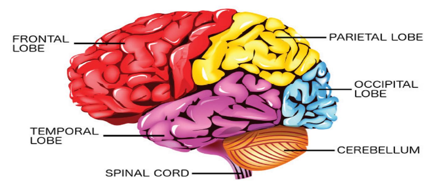
**Figure 2.** The cerebral cortex divided into the frontal, temporal, parietal, and occipital lobes [13].
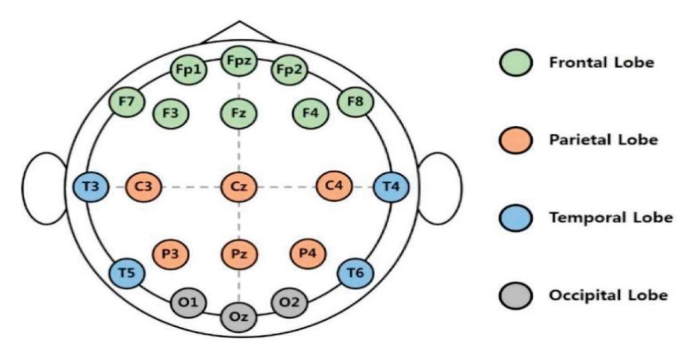
**Figure 3.** The international 10/20 system for electrode placement [14].
EEG signals are typically decomposed into five basic frequency bands which are the delta (Δ), theta (*θ*), alpha (*α*), beta (*β),* and gamma (*δ*) bands (Figure 4). Each frequency band is associated with a different type of brain activity [15–17]. Delta and theta are the two slowest brain waves often occurring whilst sleeping and during deep meditation. Specifically, delta waves are more dominant in deep restorative sleep (unconsciousness), whereas theta waves are related to light sleep, daydreaming, praying, and deep relaxation (subconsciousness). Both waves were also detected in cognitive processing, learning, and memory [17,18]. Alpha, beta, and gamma brain waves are on the other hand associated with consciousness. Alpha are the dominant brain waves of normal adults occurring when one is calm and relaxed while still being alert. Beta waves are produced throughout daily activities performed in attentive wakefulness. Gamma are the fastest waves linked to complex brain activities requiring high level of thought and focus, for example problem solving. Table 1 summarizes the five different brain wave bands and their associated psychological states. Brain wave frequency bands are typically used to extract meaningful emotion-related features [17].
Historically, EEG equipment has been highly complicated and bulky, restricted to the monitoring of stationary subjects by highly trained technical experts within controlled lab settings [19]. Recently, enormous effort has been exerted to develop wearable EEG handsets that are reliable, affordable, and portable, by that overcoming the limitations of conventional EEG headsets (Figure 5). Wearable EEG headsets allow for the long-term recording of brain signals while people are unmonitored, out of the lab, and navigating freely. Furthermore, EEG signals collected by the wearable headsets can be easily sent to 179
*Sensors* **2023**, *23*, 1255
a computer or mobile device for storage, monitoring, and/or data processing. Wearable EEG devices thus allow for the development of many clinical and non-clinical applications that were never previously possible. For example, wearable EEG has been shown to be effective for stroke [20], seizure [21], and sleep [22] remote monitoring by medical experts. EEG signals from wearable headsets can also be used for the development of brain-controlled-interface (BCI) applications such as car driver assistance [23], as well as wheelchair control for people with disability [24]. In addition, individuals can use EEG to improve their productivity and wellness via monitoring their moods and emotions [25]. However, extracting meaningful information using few EEG channels in order to reduce the computational complexity of wearable headsets is still an ongoing challenge [26,27].
| Band | Symbol | Frequency Range | | Psychological State |
|-------|--------|-----------------|-----------------|---------------------|
| Delta | Δ | <4 Hz | unconsciousness | Deep sleep |
**Table 1.** Characteristics of the five basic brain waves.
**Delta** Δ <4 Hz unconsciousness Deep sleep **Theta** *θ* 4–8 Hz subconsciousness Light sleep and meditation **Alpha** *α* 8–12 Hz consciousness Normal relaxed yet alert adult **Beta** *β* 12–30 Hz Daily activities **Gamma** *δ* >30 Hz Complex brain activities
In the present study, a subject-dependent emotional valence recognition algorithm is introduced that is intended for wearable EEG devices. The contributions of this work are as follows:
- a. Only the difference signal between the frontal Fp1 and Fp2 channels was considered for feature extraction.
- b. Simple statistical features were explored (Hjorth parameters, zero-crossings, and power spectral density), all which share the merit of having low computational complexity.
- c. Several analyses were made to determine the frequency band, time slot, and features most suitable for reliable EEG-based valence detection.
- d. The presented valence recognition algorithm outperformed several state-of-the-art methods with the added advantages of requiring only two EEG channels, a single frequency band, as well as only two simple statistical features, thus making it suitable for integration within wearable EEG devices.
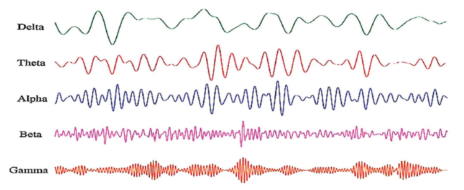
**Figure 4.** Samples from delta, theta, alpha, beta, and gamma brain waves [28].
180
*Sensors* **2023**, *23*, 1255
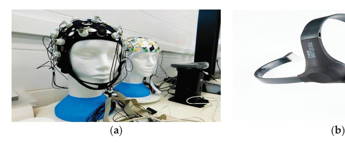
**Figure 5.** (**a**) Conventional lab EEG headset [29] versus (**b**) wearable headset from NeuroSky [30].
## 2. Literature Review
Emotion AI systems generally rely on handcrafted and/or automatic extraction of meaningful features for the classification of the different human emotional states (Figure 6). In this section, the different types of EEG-based features commonly used for emotion recognition are introduced followed by a summary of the most widely used classifiers for emotion recognition. Next, state-of-the-art EEG-based emotion detection methods from literature are presented, indicating the considered EEG channels, frequency bands, features, and the classifier, as well as the performance results.
**Figure 6.** Emotion AI system diagram.
### 2.1. EEG Features
EEG-based emotion recognition features can be categorized based on the domain from which they are computed into four different types which are as follows [31]:
- **(1) Time-domain (spatial) features** are handcrafted features that are extracted from the EEG time-series signal. They can be computed directly from the raw EEG signal or from the different frequency bands separated with the aid of bandpass filters. Time-domain features comprise simple statistical features [32–34] such as the mean, standard deviation, skewness, and kurtosis. In addition, they include more complex features such as the Hjorth parameters [5,32,35–41], High Order Crossings (HOC) [5,33,38,40,42], Fractal Dimensions [43–45], Recurrence Quantification Analysis (RQA) [46,47], in addition to entropy-based features [5,34,35,45,48].
- **(2) Frequency-domain features** are also handcrafted features, yet they are computed from the EEG signal's frequency representation. The Fast Fourier transform (FFT) and Short-time Fourier Transform (STFT) are typically used to acquire the frequencydomain signal from the EEG waves. Frequency-based features allow for the deeper understanding of the signal by considering its frequency content. Frequency-domain features include the widely used power spectral density (PSD) [33,35,39,49–51], as well as rational asymmetry features (RASM) [32,34,39,52,53]. Statistical features such as mean, median, variance, skewness, and kurtosis are also commonly computed in the EEG's the frequency domain, as well as the relative powers of the various frequency bands [54].
- **(3) Time-frequency domain features** are handcrafted features extracted from sophisticated time-frequency signal representations. Wavelet transform (WT) is a powerful tool that can decompose a signal into different subbands by applying a series of successive high and low frequency filters. WT has the advantage of being localized in
181
*Sensors* **2023**, *23*, 1255
- both time and frequency. It can thus be used to divide the EEG signal into the delta, theta, alpha, beta, and gamma subbands from which wavelet time-frequency features can be directly computed for emotion classification. Wavelet features typically include simple statistical measures such as mean, standard deviation, skewness, kurtosis, energy, and entropy [9,32,39,53,55–57].
- **(4) Deep features** refer to those features that are automatically extracted in an end-to-end manner using one or more deep networks. Deep features have been gaining increased popularity and are being used either solely or alongside handcrafted (traditional) features in emotion AI [58]. Inputs to the deep networks can be the raw EEG signal [59,60], traditional features [61], or images that are obtained either from the EEG signal's Fourier Transform (spectrograms) or Wavelet Transform (scalograms) [62–65]. In addition, the deep networks used for the feature extraction can be directly utilized or initially pretrained (transfer learning) to enhance performance.
Handcrafted (traditional) features have been widely implemented in the design of reliable EEG-based emotion AI systems. Time-domain features have the merit of being easy to implement while efficiently extracting relevant information from the EEG signals. Specifically complex time domain features such as Hjorth parameters and High Order Crossings were shown to give reliable results in EEG emotion recognition [31]. Frequencydomain features have also been widely implemented for EEG emotion recognition due to their efficient performance, yet they have the disadvantage of missing temporal information. Wavelet-domain features have the advantages of being localized in time and frequency allowing for extraction of simple yet meaningful features from the signal. A limitation of the wavelet-based features is the selection of a suitable mother wavelet [31]. Most EEG-based emotion recognition approaches thus combine different types of features for consistent performance. Several traditional classifiers were implemented in literature to classify the handcrafted features from which some of the most popular are support vector machine (SVM), k-nearest neighbor (kNN), random forests (RF), naïve Bayes (NB), and gradient boosted decision trees (GBDT) [66].
As for deep learning approaches, convolutional neural networks (CNNs), deep belief networks (DBN), and long short-term memory networks (LSTMs) among others have been used for feature extraction in emotion AI systems. In addition, pretrained readily available CNNs, such as GoogleNet, were widely used in literature as they tend to give reliable performance without requiring enormous data for training. A SVM classifier as well as sigmoid/softmax activation functions are then typically used at the network's final stage for emotion classification. Deep EEG emotion recognition methods, however, have the limitation of requiring a huge amount of data for their proper training in comparison to traditional methods [54].
### 2.2. Previous Literature
Several public EEG emotion datasets were introduced including DEAP [67], SEED [68,69], MAHNOB-HCI [70], and DREAMER [71]. Few works also report results using their own private self-generated datasets [51]. DEAP is currently considered the benchmark dataset in EEG-based emotion detection being the most widely used public EEG emotion dataset in the literature, mostly owing to it having the largest number of observations per subject [72].
EEG emotion recognition approaches can be divided into subject-dependent and subject-independent [46,73]. Subject-dependent methods train a separate model for each subject within the dataset. Subject-independent methods train a single model using data from all or some of the subjects within the considered dataset [74]. Recent papers comparing subject dependent and independent approaches showed that the former consistently gave 5–30% higher performance depending on the implemented approach. Such results are mainly due to the discrepancy between subjects related to how they feel and express their emotions [75]. For example, Nath et al. [73] have observed that EEG signals from a specific subject were somewhat similar yet significantly varied across different subjects, even when the same stimulus was considered. In addition, Putra et al. [75] found that different subjects 182
*Sensors* **2023**, *23*, 1255
varied in their response to valence stimuli, with some subjects being more responsive than others [75]. Subject-dependent approaches are thus better suited for reliable personalized emotion AI applications with wearable EEG [64].
Table 2 summarizes some of the recent EEG emotion recognition approaches using the benchmark DEAP dataset. For each research paper, the summary indicates the utilized (1) EEG channels, (2) frequency bands, (3) feature types: time—frequency—wavelet deep features, (4) classifier, (5) experimental approach: subject-dependent (*dep*.)—subjectindependent (*indep*.), as well as the (6) accuracies (*Acc*.) reported for valence (*val*.) and arousal (*arl*.) emotion recognition. For the subject independent emotion recognition methods, reported accuracies are for the experiments performed considering the complete dataset. As for the subject dependent methods, reported accuracies are the average of the experiments repeated for all the subjects in the dataset. The summarized literature review shows that subject-dependent (personalized) approaches that adopted deep learning methods, gave accuracies that were higher than 90% for both valence and arousal. However, subject-dependent approaches relying solely on traditional methods scarcely resulted in accuracies that exceeded 75%. Another limitation observed in previous literature is that most methods consider many or all EEG channel electrodes and/or frequency bands which can lead to high computational overhead with minimal, if any, performance improvement.
**Table 2.** Summary of EEG-based emotion recognition approaches that utilize the DEAP dataset.
| Research
Paper | Channels | EEG Bands | Features | Classifier | Dep./
Indep. | Val./
Arl. | Acc.
% |
|---------------------------------|-------------------------------------------------|---------------------|---------------------------------------|---------------------------|-----------------|---------------|----------------|
| Mohammadi
et al., 2017 [55] | Fp1, Fp2 | Gamma | Wavelet Features | kNN | Indep. | Val.
Arl. | 80.68
74.60 |
| | Fp1, Fp2, F7, F8, F3, F4,
FC5, FC6, FC1, FC2 | | | | | | Val.
Arl. |
| Salma et al.,
2017 [59] | All | Raw | Deep Features
(LSTM) | Sigmoid | Dep. | Val.
Arl. | 85.45
85.65 |
| Wu et al., 2017
[53] | Fp1, Fp2 | All | Frequency, WT
Features | GBDT | Dep. | Val.
Arl. | 75.18 |
| Zhuang et al.,
2017 [76] | FP1, FP2, F7, F8, T7,
T8, P7, P8 | Beta, Gamma | Time (EMD) | SVM | Dep. | Val.
Arl. | 69.10
71.99 |
| Eun et al.,
2018 [77] | Fp1, Fp2, F3, F4, T7,
T8, P3, P4* | Raw | Deep Features
(LSTM) | Sigmoid | Indep. | Val.
Arl. | 78.00
74.65 |
| | All | All except
delta | Wavelet Features | kNN | Dep. | Val.
Arl. | 59.00
65.70 |
| Putra, 2018 [75] | All | All except
delta | Wavelet Features | kNN | Indep. | Val.
Arl. | 58.90
64.30 |
| Yang et al.,
2018 [60] | All | Raw | Deep Features
(LSTM, CNN) | Softmax | Dep. | Val.
Arl. | 90.80
91.03 |
| Parui et al.,
2019 [36] | All | Raw | Time, WT Features | XGBoost | Indep. | Val. | 75.97 |
| | All | All | Frequency Features | | | Arl. | 74.20 |
| Xing et al.,
2019 [78] | All | All except
delta | Frequency Features | LSTM | Indep. | Val.
Arl. | 81.10
74.38 |
| Cui et al.,
2020 [79] | Symmetric Channels | All except
delta | Regional
Asymmetric CNN
(RACNN) | Softmax | Dep. | Val.
Arl. | 96.65
97.11 |
| Garg and
Verma,
2020 [65] | All | Raw | Scalogram Images | GoogleNet
(pretrained) | Indep. | Val.
Arl. | 92.19
61.23 |
183
*Sensors* **2023**, *23*, 1255
**Table 2.** *Cont.*
| Research
Paper | Channels | EEG Bands | Features | Classifier | Dep./
Indep. | Val./
Arl. | Acc.
% |
|------------------------------|--------------------------------|-----------------------|-----------------------------------|-----------------------------------|-----------------|---------------|----------------|
| Nath et al.,
2020 [73,80] | All | All | Band Power | LSTM | Dep. | Val.
Arl. | 94.69
93.13 |
| | | | | SVM | Indep. | Val.
Arl. | 72.19
71.25 |
| Aslan,
2021, [62] | All | Raw | Scalogram Images | GoogleNet
(pretrained)
+SVM | Indep. | Val.
Arl. | 91.20
93.70 |
| Ozdemir et al.,
2021 [81] | All | Alpha, Beta,
Gamma | Multi-Spectral
Topology Images | CNN, LSTM +
Softmax | Indep. | Val.
Arl. | 90.62
86.13 |
| Huang,
2021 [61] | Symmetric Channels | Raw signal | Bi-hemisphere
spatial features | CNN | Dep. | Val.
Arl. | 94.38
94.72 |
| | | | | | Indep. | Val.
Arl. | 68.14
63.94 |
| Yin et al.,
2021 [48] | All | Raw signal | Differential Entropy
Cube | GCNN,
LSTM | Dep. | Val.
Arl. | 90.45
90.60 |
| | | | | | Indep. | Val.
Arl. | 84.81
85.27 |
| Zhang et al.,
2021 [58] | Fp1, Fp2, F3,
F4, AF3, AF4* | All | Time, Frequency | Softmax | Indep. | Val.
Arl. | 84.71
83.28 |
| Cheng et al.,
2022 [82] | All | Raw Signal | Deep Features
(randomized CNN) | Ensemble | Dep. | Val.
Arl. | 99.19
99.25 |
| Gao et al.,
2022 [37] | All | All except
delta | Time, Frequency
Features | CNN
+ SVM | Indep. | Val.
Arl. | 80.52
75.22 |
In the present study, a subject-dependent approach is adopted for valence (happy/sad) emotion classification intended for personalized emotion AI applications with wearable EEG. Since several previous studies showed that the frontal channels are the most relevant for EEG-based emotion recognition [33,39,40,53,83], only the Fp1 and Fp2 channels were considered for emotion recognition. The widely used DEAP benchmark dataset was considered for its reliability, as well as to facilitate comparison to previous approaches. Time and frequency EEG features were extracted from a single time series related to the Fp1 and Fp2 channels which are the Hjorth parameters, zero-crossings, and PSD.
Happiness and sadness emotions (valence) have been reported to dramatically affect the theta, alpha, and beta waves of the frontal channels [84]. Interestingly, the delta [85], alpha [86], and gamma [87,88] waves of the frontal channels were also shown to be individually useful for EEG-based emotion recognition. Several analyses were thus performed in this work to determine the frequency bands most suitable for valence detection considering the different computed features. In addition, performance was observed when the compete EEG signal was considered for feature computation in comparison to when only a short segment was utilized. The aim of the performed analyses was to find the most suitable feature set that would achieve superior performance comparable to state-of the-art methods, all while requiring minimal computational overhead. Primarily, only the sixteen strongest emotions (eight happiest and eight saddest) were considered in the analyses in order to assure significant discrepancy between the emotions. Then, the complete DEAP dataset was utilized for the final experimentations concerning binary and multiclass valence classifications, as well as for comparison to previous literature.
184
*Sensors* **2023**, *23*, 1255
## 3. Methods
### 3.1. Dataset
DEAP is a public audio-visual stimuli-based emotion dataset [67] that was collected from 32 subjects. For emotion recognition, the use of audio-visual stimuli guarantee higher valence intensity is experienced with respect to visual stimuli (pictures) [89]. The subjects ages ranged between 19 and 37, with an average of 26.9 years. Each subject watched 40 one-minute music videos intended to elicit different emotions. These one-minute videos were extracted from long-version music videos to include maximum emotional content. EEG signals from thirty-two electrodes placed according to the international 10/20 system were recorded at a sampling rate of 512 Hz then downsampled to 128 Hz. Each electrode recorded 63 s EEG signal, with a 3s baseline signal before the trial. The 3 s baseline was ignored here as previously performed in [58,76,77,90].
After watching each video, participants performed a self-assessment of their emotional states of valence, arousal, liking, and dominance on a continuous scale from 1 to 9. Only valence was considered in the present study which would be useful for personalized medical applications as well as in emotion-based entertainment content. The valence scale ranges from sad to happy with ratings closer to one representing low valence (sad), whereas ratings closer to nine indicating high valence (happy). For the binary classification experiments, a threshold (*thresh*.) of five was considered to separate the low and high valence classes as commonly performed in many other works such as Refs. [58,60,61,73,74,76,77,91–94]. This threshold value is typically chosen to overcome the class imbalance issue in the DEAP dataset [64,67]. As for the three-class classifications, thresholds of three and six were considered to divide the dataset into low valence (sad), mid-range (neutral), and high valence (happy).
### 3.2. Channel Selection
The international 10/20 system includes several electrode placement markers applied to detect the brain waves from the different brain lobes. In deep learning approaches where it is basically the network's task to extract meaningful features from the data, it is common to input all the EEG channels to the network for emotion recognition [59,60,94]. Nevertheless, several studies have shown that considering all EEG channels can be redundant and that extracting features from a few significant channels can results in reliable performance with the added advantage of reduced computational complexity [35,53,55].
For wearable EEG headsets, requiring only one or two EEG channels can substantially reduce the hardware complexity thus facilitating its usage in non-laboratory settings, as well as reducing its overall cost, all which would make it more attractive to day-to-day consumers [35,53,95]. From the different brain lobes, the frontal lobe is the one most associated with emotion recognition using EEG signals [5]. Specifically, several studies have shown that features calculated from the prefrontal brain region (Fp1-Fp2) result in best performance as compared to other brain areas [35]. Mohammadi et al. [55] more specifically showed that the Fp1-Fp2 channel pair resulted in highest accuracies in comparison to other frontal channel pairs, and that combining all the frontal channels resulted in a somewhat enhanced performance. Interestingly, Wu et al. [53] found that not only did Fp1-Fp2 result in the highest accuracies in comparison to the other frontal channels, but that solely using Fp1-Fp2 resulted in similar performance to the case when features from four or six frontal channels were combined. The Fp1-Fp2 channel pair was thus chosen in this study for valence-related feature extraction.
Previous research has shown that positive emotions are associated with left frontal activity, whereas negative emotions are associated with right frontal activity [96,97]. Symmetric channel pairs from the left and right brain hemispheres were thus commonly considered in literature by being either subtracted or divided in order to create a single wave from which relevant features were calculated [61,98,99]. In the present study, the EEG features were extracted from a single time series signal computed as the difference between
185
*Sensors* **2023**, *23*, 1255
the Fp1 and Fp2 channels in order to measure the asymmetry in brain activity due to the valence emotional stimuli [67].
### 3.3. EEG Band Separation
Five different third order Butterworth band-pass filters were implemented to separate the delta (2–4 Hz), theta (4–8 Hz), alpha (8–12 Hz), beta (12–30 Hz), and gamma (30–60 Hz) frequency bands (Table 1). The Butterworth filter has been previously used for the EEG bands separation owing to its flat response, simplicity, and efficiency [5,40].
## 3.4. Feature Extraction
Both time and frequency domain EEG features were initially computed from all the frequency bands (delta–theta–alpha–beta–gamma). Next, feature analysis was performed to determine which features were more suitable for valence emotion recognition, as well as the most relevant frequency band for feature extraction.
### A. Hjorth Parameters
Hjorth parameters [100] were introduced by Bo Hjorth in 1970 to represent several signal statistical properties (Figure 7). Hjorth parameters have been successfully used in various EEG emotion recognition research [5,32,35–40]. The three Hjorth parameters are activity (variance), mobility, and complexity given by the following equations:
$$Activity = \operatorname{Var}(y(t)) \quad (1)$$
Mobility =
$$\sqrt{\frac{activity(\frac{dy(t)}{dt})}{activity(y(t))}}$$
(2)
$$Complexity = \sqrt{\frac{mobility(dy(t)/dt)}{mobility(y(t))}} (3)$$
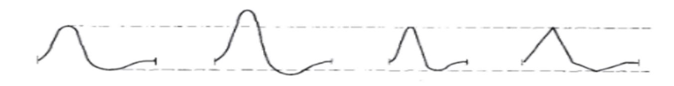
**Figure 7.** Characteristic changes in an arbitrary reference signal, illustrating their relation to the different Hjorth parameters [100].
### B. Zero-Crossings
The zero-crossings of a signal are the number of times the signal intercepts the horizontal x-axis thus changing signs. Zero crossings are used to measure the oscillating property of a signal indicating the degree of excitation within a specific frequency band.
### C. Power Spectral Density
Power spectral density (PSD) is among the most widely implemented EEG features for emotion recognition [72]. PSD describes the average signal power over its frequency bands. To obtain the PSD, the amplitude of the FFT is multiplied by its complex conjugate which is then summed to get the total power.
## 4. Results
In the present study, an EEG-based subject-dependent valence emotion recognition approach is presented using the difference Fp1-Fp2 signal. Figure 8 illustrates the experimental workflow adopted in order to develop an efficient and reliable system that is suitable for wearable EEG. Initially, the Hjorth parameters (activity–mobility–complexity), zero-crossing, and PSD features were computed from the different frequency bands. Next, 186
*Sensors* **2023**, *23*, 1255
the strongest emotions per subject were considered for the feature analyses in which the EEG bands, timeslots, and features were determined. Finally, the selected feature set was used for the binary and multiclass valence emotion classification of the complete DEAP dataset. Since a subject dependent approach was adopted in this work, all the classification experiments were repeated for each of the 32 subjects in the DEAP dataset, and the average accuracies of all subjects were reported as the final performance measure.
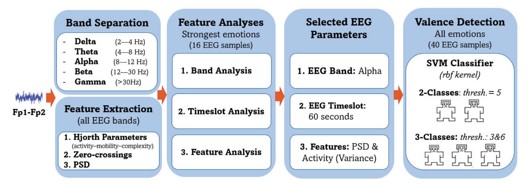
**Figure 8.** Experimental workflow.
KNN and SVM classifiers are the most commonly used for EEG emotion recognition [66,72]. The kNN classifier has the advantages of being simple while giving reliable results [45]. The SVM classifier can be easily tuned for optimal performance. A kNN classifier was used for the feature analyses, whereas both the kNN and SVM with radial basis function (rbf) were considered in the final classification experiments. For the kNN classifier, several k values were compared, then k = 5 was chosen as it was found to give better overall performance. For all cases, the Euclidian distance was considered within the kNN classifier to determine the nearest neighbors. As for the SVM classifier, the hyperparameters (cost and gamma) were repeatedly tuned for each subject in the different experiments using Bayesian optimization. A leave-one-out cross-validation (LOOCV) was used in all the experiments. All feature computations and classification experiments were performed using MATLAB R2021a on an Intel Core i7-5500U CPU @2.4 GHz with 16 GB of RAM.
### 4.1. Feature Analyses
In this work, the aim of the feature analyses was to determine the most relevant (1) frequency band (delta–theta–alpha–beta–gamma), (2) timeslot (first 20 s–middle 20 s– last 20 s–complete 60 s), and (3) features (activity–mobility–complexity–zero-crossings– PSD) for EEG valence recognition. Sixteen videos per subject were included in the feature analyses, those being the ones with eight highest and eight lowest self-rated valence emotions. Considering only the strongest emotions assures significant discrepancy between the two emotional classes (high valence and low valence) for more reliable feature analyses. A similar approach was previously considered in [52,53].
## A. Band/Feature Analysis
Feature/band analysis was performed in order to determine the frequency bands and features most suitable for valence classification. The three Hjorth parameters, zerocrossings, and PSD features were calculated from the five EEG frequency bands (delta, theta, alpha, beta, gamma). KNN classifier was then used to classify the 1 minute trials into high or low valence. Figure 9 summarizes the valence (happy/sad) classification performance for the different experiments. For all the EEG frequency bands, the variance
187
*Sensors* **2023**, *23*, 1255
(Hjorth activity) and PSD were found to result in the highest accuracies. Roshdy et al. [101] have previously shown that the standard deviation, which is the square root of the variance, was highly correlated with valence emotion. PSD is among the most widely accepted measure for valence recognition in the literature [102]. Results of the feature analysis are thus in agreement with previous literature.
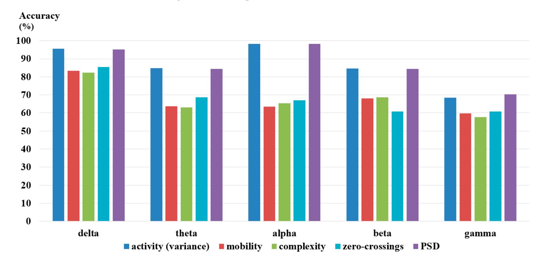
**Figure 9.** Valence classification accuracies for the different features and EEG frequency bands.
Table 3 summarizes the variance and PSD accuracies for the five different frequency bands. Results indicate that for both features, the alpha band gave the most reliable performance closely followed by the delta band. These results are in agreement with several research that showed that the alpha [32,72] and delta [85] bands were relevant for valence emotion detection. The low accuracies attained by the gamma band features were however unconventional as the gamma band was previously shown to be suitable for emotion recognition [55,87]. The gamma band was thus further divided into three subbands which are 30–40 Hz, 40–50 Hz, and 50–60 Hz, and the previous analysis were repeated. Results summarized in Table 4 indicate a significant improvement in performance when the gamma band was subdivided into three different subbands. Best results were attained by the fast gamma subband (50–60 Hz) for which accuracies of 99.02% and 98.63% were achieved for the variance and PSD, respectively, by that outperforming results attained by the same features for the delta and alpha bands.
**Table 3.** Valence classification accuracies (%) for the different EEG bands using activity and PSD.
| | All
(2–60 Hz) | Delta
(2–4 Hz) | Theta
(4–8 Hz) | Alpha
(8–12 Hz) | Beta
(12–30 Hz) | Gamma
(30–60 Hz) |
|----------|------------------|-------------------|-------------------|--------------------|--------------------|---------------------|
| variance | 62.50 | 95.51 | 84.77 | 98.24 | 84.57 | 68.56 |
| PSD | 61.33 | 95.12 | 84.38 | 97.85 | 84.38 | 70.31 |
**Table 4.** Valence classification accuracies (%) for the different gamma subbands using activity and PSD.
| | 30–60 Hz | 30–40 Hz | 40–50 Hz | 50–60 Hz |
|----------|----------|----------|----------|----------|
| variance | 68.56 | 91.99 | 91.40 | 99.02 |
| PSD | 70.31 | 91.99 | 91.02 | 9.63 |
188
*Sensors* **2023**, *23*, 1255
Based on the feature/band analysis, it can be deduced that the variance (Hjorth activity) and PSD calculated from the delta, alpha, and fast gamma frequency bands result in the most consistent performance. Further experiments performed in this study will thus only use the indicated features and frequency bands.
### B. Time Slot Analysis
In the DEAP dataset, a 1 minute EEG recording is provided for each video stimulus per subject. Several previous works considered only the middle time slot omitting the first part for emotions to settle and the last part for fatigue [56,58]. Others used only the last thirty seconds under the assumption that it yields better results [53,67]. In order to test these presumptions, the variance (Hjorth activity) and PSD features were calculated from the first, middle, and last 20 seconds (s) of the EEG recordings for the delta, alpha, and fast gamma bands. Valence classification results for the three indicated timeslots in comparison to using the complete 1 minute are summarized in Table 5. Overall, better valence classification performance is achieved by the alpha and fast gamma bands (~97–99%) than for the delta band (~95–96%). For the delta band, results from the different slots were somewhat close. However, the first timeslot resulted in slightly improved results compared to when the complete 1 minute was considered. As for the alpha and fast gamma bands, results indicate that the middle time slot gave more reliable performance in comparison to the first and last timeslots. Nevertheless, considering the full 1 minute EEG signal resulted in an overall better performance than for any of the 20 s time slots. The full one-minute signal will thus be considered for more consistent performance in all the upcoming experiments.
**Table 5.** Strongest emotion classification accuracies (%) for different EEG time slots.
| | Delta (2–4 Hz) | | Alpha (8–12 Hz) | | Gamma (50–60 Hz) | |
|---------|----------------|--------------|-----------------|--------------|------------------|--------------|
| | Variance | PSD | Variance | PSD | Variance | PSD |
| 1–20 s | 96.29 | 96.09 | 97.46 | 97.07 | 97.66 | 97.66 |
| 20–40 s | 95.51 | 95.70 | 97.46 | 97.46 | 98.05 | 98.05 |
| 40–60 s | 94.92 | 95.51 | 96.68 | 97.27 | 98.05 | 97.85 |
| 1–60 s | 95.51 | 95.12 | 98.24 | 98.24 | 99.02 | 98.63 |
### C. Feature Boxplots
At the beginning of this section, the activity (variance), mobility, complexity, zerocrossings, and PSD features were computed from the five EEG frequency bands. Classification results considering the strongest emotions showed that the variance and PSD were the most relevant for valence emotion recognition regardless of the frequency band. Specifically, experimentation results showed that the variance and PSD computed from the delta, alpha, and fast gamma full 1 minute EEG signals resulted in the most reliable valence emotion classification performance in comparison to the other considered cases.
In this subsection, the boxplots of the variance and PSD were generated (Figure 10) to illustrate the features' distributions for the two valence classes: low valence (sad) and high valence (happy). Boxplots display a five-number summary of the data including the minimum, first quartile, second quartile (median), third quartile, and maximum. For both features, the boxplots demonstrate significant discrepancy between the two valence classes which emphasizes their relevance as previously shown in the different classification experiments within the previous subsections.
189
*Sensors* **2023**, *23*, 1255
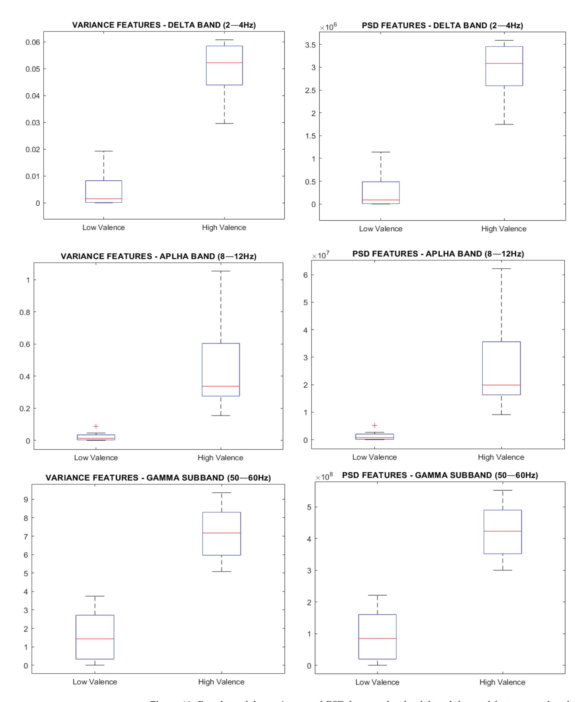
**Figure 10.** Boxplots of the variance and PSD features for the delta, alpha, and fast gamma bands considering the full 1 minute EEG signal.
190
*Sensors* **2023**, *23*, 1255
### 4.2. Valence Classifications
In this section, the subject dependent valence emotion classifications were performed considering all the forty video trials included in the DEAP dataset. The variance (Hjorth activity) and PSD features were computed from the full 1 minute delta, alpha, and fast gamma bands which were found in the previous section to be the most relevant for valence classification. Variance and PSD were used both individually and collectively and results were given for each case. KNN and SVM with rbf kernel were considered in all experiments.
Tables 6 and 7 summarize the binary classification accuracies for the kNN and SVM classifiers, respectively. Overall, the SVM classifier gave better accuracies than the kNN classifier. The alpha band is shown to give consistently better results closely followed by the delta band, whereas the fast gamma band results are almost 10% less for both classifiers. Fast gamma is thus shown to be reliable when discriminating between strong sad and happy emotions attaining accuracies that were as high as 99% (Table 4), yet less useful when more mellow emotional states were additionally involved.
**Table 6.** Valence classification accuracies (%) for the complete DEAP dataset (kNN).
| | Delta
(2–4 Hz) | Alpha
(8–12 Hz) | Fast Gamma
(50–60 Hz) |
|----------------|-------------------|--------------------|--------------------------|
| Variance | 95.08 | 96.09 | 85.23 |
| PSD | 95.08 | 96.25 | 84.76 |
| Variance + PSD | 95.00 | 96.33 | 85.55 |
**Table 7.** Valence classification accuracies (%) for the complete DEAP dataset (SVM-rbf).
| | Delta
(2–4 Hz) | Alpha
(8–12 Hz) | Fast Gamma
(50–60 Hz) |
|----------------|-------------------|--------------------|--------------------------|
| Variance | 96.95 | 97.26 | 87.58 |
| PSD | 95.55 | 96.80 | 87.50 |
| Variance + PSD | 97.19 | 97.42 | 87.11 |
Generally, variance (Hjorth activity) and PSD gave close results in all experiments. For the alpha and delta bands, all achieved accuracies were greater than or equal to 95%, indicating the efficacy of the considered features for valence emotional recognition. Variance did, however, give slightly better results than PSD in most cases. Combining these two features resulted in an overall more consistent performance. Best results were achieved when the combined features were calculated from the alpha band resulting in accuracies of 96.33% and 97.42% for the kNN and SVM classifiers, respectively. Several research has shown that the frontal channels' alpha band was significantly affected by a person's happiness and sadness emotions [28,103]. The findings of this work, in which the alpha band was found to be more reliable than other frequency bands for valence recognition, are thus in agreement with previous literature.
For the sake of attaining a more comprehensive insight on the performance of the proposed method, the valence classification accuracies per subject for the combined variance and PSD features for the delta, alpha, and fast gamma bands are presented in Table 8. For the alpha band, twenty-eight and thirty of the total thirty-two DEAP subjects had their emotions recognized with an accuracy that is greater than or equal to 95% for the kNN and SVM classifiers, respectively, which indicates the reliability of the considered features.
191
*Sensors* **2023**, *23*, 1255
**Table 8.** Valence classification accuracies (%) per subject for the combined variance and PSD features considering the complete DEAP dataset.
| | kNN | | | SVM (rbf) | | |
|---------|-------|-------|------------|-----------|-------|------------|
| Subject | Delta | Alpha | Fast Gamma | Delta | Alpha | Fast Gamma |
| 1 | 95.0 | 97.5 | 77.5 | 97.5 | 97.5 | 77.5 |
| 2 | 92.5 | 95.0 | 77.5 | 87.5 | 95.0 | 82.5 |
| 3 | 95.0 | 97.5 | 72.5 | 97.5 | 97.5 | 75.0 |
| 4 | 100 | 92.5 | 60.0 | 97.5 | 95.0 | 72.5 |
| 5 | 95.0 | 90.0 | 90.0 | 97.5 | 95.0 | 92.5 |
| 6 | 100 | 95.0 | 97.5 | 100 | 97.5 | 95.0 |
| 7 | 95.0 | 95.0 | 87.5 | 97.5 | 100 | 92.5 |
| 8 | 95.0 | 97.5 | 77.5 | 97.5 | 100 | 85.0 |
| 9 | 95.0 | 97.5 | 82.5 | 97.5 | 97.5 | 87.5 |
| 10 | 95.0 | 97.5 | 90.0 | 100 | 95.0 | 90.0 |
| 11 | 90.0 | 92.5 | 90.0 | 90.0 | 95.0 | 87.5 |
| 12 | 95.0 | 100 | 85.0 | 100 | 100 | 85.0 |
| 13 | 97.5 | 95.0 | 70.0 | 100 | 97.5 | 67.5 |
| 14 | 95.0 | 97.5 | 97.5 | 100 | 97.5 | 100 |
| 15 | 95.0 | 97.5 | 82.5 | 97.5 | 97.5 | 82.5 |
| 16 | 100 | 95.0 | 75.0 | 100 | 95.0 | 77.5 |
| 17 | 95.0 | 97.5 | 85.0 | 97.5 | 100 | 85.0 |
| 18 | 97.5 | 100 | 90.0 | 97.5 | 100 | 92.5 |
| 19 | 95.0 | 95.0 | 95.0 | 97.5 | 92.5 | 95.0 |
| 20 | 95.0 | 97.5 | 85.0 | 97.5 | 97.5 | 90.0 |
| 21 | 95.0 | 97.5 | 90.0 | 100 | 97.5 | 97.5 |
| 22 | 97.5 | 100 | 90.0 | 100 | 100 | 85.0 |
| 23 | 92.5 | 100 | 95.0 | 95.0 | 100 | 95.0 |
| 24 | 97.5 | 97.5 | 77.5 | 95.0 | 97.5 | 77.5 |
| 25 | 95.0 | 95.0 | 87.5 | 97.5 | 97.5 | 85.0 |
| 26 | 95.0 | 95.0 | 100 | 97.5 | 97.5 | 100 |
| 27 | 97.5 | 90.0 | 95.0 | 100 | 92.5 | 95.0 |
| 28 | 87.5 | 97.5 | 97.5 | 90.0 | 97.5 | 97.5 |
| 29 | 95.0 | 95.0 | 97.5 | 97.5 | 95.0 | 97.5 |
| 30 | 95.0 | 97.5 | 87.5 | 97.5 | 100 | 90.0 |
| 31 | 85.0 | 97.5 | 82.5 | 92.5 | 100 | 85.0 |
| 32 | 95.0 | 97.5 | 70.0 | 100 | 100 | 70.0 |
| Average | 95.0 | 96.33 | 85.55 | 97.19 | 97.42 | 87.11 |
In order to further investigate these results, the median, average, and standard deviation of the valence ratings of the two subjects with the lowest and highest SVM accuracies in the alpha band were inspected and summarized in Table 9. Furthermore, these statistical measures were also calculated for all the thirty-two subjects in the DEAP dataset. For subject #27 (one of the subjects with the lowest accuracies), it is noticed that both the median and average of the valence ratings are higher than the value of the threshold considered in this work for the low/high valence class separation. Modifying this threshold value
192
*Sensors* **2023**, *23*, 1255
to become six instead of five, which is closer to subject #27's median and average, indeed resulted in improving this subject's emotional recognition accuracy by 5% to become 97.5%. On the other hand, the increased threshold had no effect or minimal effect on the other considered subjects and minimal effect on the overall performance. These results indicate the robustness of the two implemented measures for valence emotion recognition whilst also highlighting the importance of considering subject variability for more reliable results.**Table 9.** Valence ratings statistical measures and classification accuracies for different valence thresholds, given for the subjects with the lowest and highest performance as well as for the complete DEAP dataset.
| | | Highest Accuracies | | Lowest Accuracies | | All Subjects |
|--------------------------------------------|----------------|--------------------|----------------|-------------------|----------------|--------------|
| | | Subject
#12 | Subject
#22 | Subject
#19 | Subject
#27 | |
| Valence ratings
statistical
measures | Median | 5.04 | 5.00 | 5.04 | 6.08 | 5.04 |
| | Average | 4.88 | 4.69 | 5.23 | 6.08 | 5.25 |
| | Std. deviation | 2.24 | 2.44 | 1.80 | 2.18 | 2.13 |
| Accuracies
(SVM) | Threshold = 5 | 100 | 100 | 92.5 | 92.5 | 97.42 |
| | Threshold = 6 | 97.5 | 100 | 92.5 | 97.5 | 96.56 |
Table 10 summarizes the three-class valence classification results using the variance, PSD, as well as both features calculated from the delta, alpha, and fast gamma bands. Similar to the binary classifications, best results were attained when the features were computed from the alpha band, closely followed by the delta band. For the alpha and delta bands, considering one of the features or both combined resulted in close accuracies ranging from 94.22% to 95.39%. Best performance (accuracy = 95.39%) was attained when the variance was computed from the alpha band.
**Table 10.** Valence three-class accuracies (%) for the complete DEAP dataset (SVM-rbf).
| | Delta
(2–4 Hz) | Alpha
(8–12 Hz) | Fast Gamma
(50–60 Hz) |
|----------------|-------------------|--------------------|--------------------------|
| Variance | 94.30 | 95.39 | 78.13 |
| PSD | 94.69 | 94.22 | 78.28 |
| Variance + PSD | 94.92 | 95.00 | 78.44 |
## 5. Discussion
In the present study, an efficient EEG-based valence recognition method was presented that considers only the difference Fp1-Fp2 signal for feature extraction. Analyses showed that the variance and PSD computed from the 1 minute alpha band were the most suitable for valence recognition. Final classification experiments considering the entire DEAP dataset resulted in accuracies of 97.42% and 95.39% for the two and three class valence classifications, respectively. Torres et al. [72] have reported that in previous literature, accuracies were on average about 85% and 68% for two and three class EEG-based valence classifications, respectively. The performance of the proposed methods thus surpasses the average performance of EEG-based valence detection methods by approximately 10% and 27% for two- and three-class classifications, respectively, indicating the superiority of the implemented method.
The notion that few simple handcrafted features can give promising results in EEGbased valence classification has been previously demonstrated in several research papers. In an early work by Sourina et al. [104], accuracies well above 90% were achieved for all subjects considering only three frontal channels using music to invoke the emotional stimuli. 193
*Sensors* **2023**, *23*, 1255
In another work by Amin et al. [105], emotion recognition accuracies exceeding 98% were attained considering only the relative wavelet energy, which was calculated from the delta band of 128 electrodes. However, for both these works performance could not be compared to other methods as private datasets were utilized. A later work by Thejaswini et al. [32] achieved an overall average accuracy of 91.2% upon classifying the SEED dataset to three classes: positive, neutral, and negative emotions. They implemented simple statistical features including the RASM and Hjorth parameters, but again considering twenty-seven electrode pairs for the feature computations.
The DEAP dataset, considered in this study, is reportedly the most widely utilized for EEG emotional recognition [72] which facilitates comparison between the different approaches. Table 11 summarizes the performance of several other EEG emotion recognition methods from literature that also used the DEAP dataset. The comparison indicates the EEG channels and frequency bands considered in each approach, as well as the binary classification accuracy. For the sake of a fair comparison, all valence emotion recognition methods included are based on subject-dependent experiments, which is the approach considered in this work. Wu et al. [53], like in this work, used only the FP1 and Fp2 frontal channels, yet achieved a relatively low accuracy of 75.18%. Other methods used all the EEG channels whether individually or in the form of channel pairs. In addition, most of the studies summarized in Table 11 considered all the frequency channels by that ignoring the significance of some bands over others for valence emotion recognition. Overall, the valence classification accuracies of the summarized approaches mostly range from 75.18% to 96.65%. The EEG valence emotion recognition method introduced in the present study results in an accuracy of 97.42% by that outperforming several state-of-the-art methods deep learning methods.
**Table 11.** Valence (happy/sad) classification performance for the DEAP dataset.
| Method | Year | Method | Channels | Bands | Acc. % |
|-------------------|------|-----------------------------------|-------------------------|------------------|--------|
| Wu et al. [53] | 2017 | FFT and WT features with GBDT | Fp1, Fp2 | All | 75.18 |
| Salma et al. [59] | 2017 | LSTM and RNN | All | Raw | 85.45 |
| Yang et al. [60] | 2018 | LSTM and CNN | All | All | 90.80 |
| Cui et al. [79] | 2020 | Differential Entropy + SVM | Symmetric channel pairs | All except delta | 89.09 |
| | | Multilayer Perceptron (MLP) | | | 92.57 |
| | | Regional-Asymmetric CNN (RACNN) | | | 96.65 |
| Nath et al. [80] | 2020 | Band power with LSTM | All | All | 94.69 |
| Yin et al. [48] | 2021 | Differential entropy with ECLGCNN | All | All | 80.52 |
| Huang et al. [61] | 2021 | Bi-hemisphere discrepancy CNN | Symmetric channel pairs | Raw | 94.38 |
| Chen et al. [82] | 2022 | Ensemble Deep Randomized-CNN | All | Raw | 99.19 |
| Proposed | 2022 | Variance + PSD with SVM | Fp1-Fp2 | Alpha | 97.42 |
Nevertheless, the recent approach introduced by Cheng et al. [82], which is based on randomized CNN and ensemble learning, resulted in an overall accuracy of 99.17% which is 1.75% higher than the implemented method. In their work, they reported an average training time of 35.15 s. As for the proposed method, an average of 0.06 s were required for the feature computation, training, and classification. Nevertheless, the machine learning-based proposed approach, even though performing not as well as Cheng et al.'s method, has the valuable merit of being simpler to reproduce.
The proposed EEG-based valence emotion recognition method was shown to result in reliable performance while relying on statistical measures that are simple to compute. In addition, it relies on standard machine learning algorithms that are easily configured. No image construction was required, and no complex neural networks needed to be trained. In 194
*Sensors* **2023**, *23*, 1255
the literature, several works have also shown that handcrafted features can achieve comparable performance to deep learning approaches with the former having the merit of reduced computational complexity which could be attractive in real-time applications [106–108]. Another advantage of the presented method is that unlike in other literature where all the frequency bands or the raw EEG signal were considered, only the alpha band was used for feature extraction. The alpha band was utilized in this work as it was shown in the analyses performed in Section 4.1 to be the most relevant for valence detection. Interestingly, several clinical studies have previously shown that there is indeed a relationship between the alpha activity measured from the prefrontal cortex and emotional response [109,110].
The proposed method considers only the Fp1-Fp2 channel pair from which the alpha band's variance and PSD were computed, by that minimizing the computational overhead whilst achieving reliable performance making it suitable for wearable EEG headsets used in real-time applications [26,111]. Overall, the results attained here are quite promising. Yet, there is still room for enhancement of the suggested method. Future work includes considering arousal along with valence recognition, as well as calculating other statistical features that are relevant to EEG-based emotion recognition such as entropy and RASM. In addition, the integration of handcrafted and deep features can be investigated. Explainable AI (XAI) methods can then be implemented to understand what the models are learning and why the specific decisions were made. XAI can also be applied to investigate whether EEG-based emotion detection is gender or culture dependent, as is speech emotion recognition [112].
## 6. Conclusions
EEG-based subject-dependent valence emotion recognition is widely implemented in personalized emotion AI applications. In this work, the difference signal (Fp1-Fp2) was used to calculate the Hjorth parameters (variance-mobility-complexity), zero-crossings, and PSD features for the emotional valence detection using the benchmark DEAP dataset. Several analyses were performed to determine the features, frequency band, and timeslot most suitable for reliable subject-based valence recognition. Primarily, only the eight strongest high and low valence emotions per subject were considered for analysis to assure significant discrepancy between the two classes. Classification results indicated that the variance and PSD features were the most suitable for valence recognition regardless of the considered frequency channel. Nevertheless, the delta, alpha, and fast gamma bands were shown to be the most relevant for valence recognition. Boxplots of the variance and PSD features for the most relevant frequency bands validated and supported the classification results. In addition, calculating the features from the complete 1 minute EEG signal was found to give more reliable performance than when only a 20 s timeslot was used for feature computation. Best results were achieved when the variance and PSD were computed from the alpha band resulting in accuracies of 97.42% and 95.0% for the binary and multiclass classification, respectively. Comparison to previous literature showed that implemented method outperformed several state-of-the-art approaches with the advantage of reduced computational complexity due to the reduced number of electrodes, features, and frequency bands considered. This approach would thus be highly attractive for practical EEG-based emotion AI systems relying on wearable EEG devices.
**Funding:** This research received no external funding.
**Institutional Review Board Statement:** Not applicable.
**Informed Consent Statement:** Not applicable.
**Data Availability Statement:** The DEAP dataset supporting reported results is a public dataset that can be found here: https://www.eecs.qmul.ac.uk/mmv/datasets/deap/download.html, accessed on 16 January 2023.
**Conflicts of Interest:** The author declares no conflict of interest.
195
*Sensors* **2023**, *23*, 1255
### References
- 1. Meredith Somers. Emotion AI, Explained. 2019. Available online: https://mitsloan.mit.edu/ideas-made-to-matter/emotion-aiexplained (accessed on 21 May 2022).
- 2. Charlotte Gifford. The Problem with Emotion-Detection Technology. 2020. Available online: https://www.theneweconomy.com/ technology/the-problem-with-emotion-detection-technology (accessed on 21 May 2022).
- 3. Ekman, P.; Friesen, W.V. Constants across cultures in the face and emotion. *J. Pers. Soc. Psychol.* **1971**, *17*, 124. [CrossRef]
- 4. Russell, J.A. A circumplex model of affect. *J. Personal. Soc. Psychol.* **1980**, *39*, 1161–1178. [CrossRef]
- 5. Shashi Kumar, G.S.; Sampathila, N.; Shetty, H. Neural Network Approach for Classification of Human Emotions from EEG Signal. In *Engineering Vibration, Communication and Information Processing*; Ray, K., Sharan, S., Rawat, S., Jain, S., Srivastava, S., Bandyopadhyay, A., Eds.; Springer Singapore: Singapore, 2019; pp. 297–310.
- 6. Tsiourti, C.; Weiss, A.; Wac, K.; Vincze, M. Multimodal Integration of Emotional Signals from Voice, Body, and Context: Effects of (In)Congruence on Emotion Recognition and Attitudes Towards Robots. *Int. J. Soc. Robot.* **2019**, *11*, 555–573. [CrossRef]
- 7. Canal, F.Z.; Müller, T.R.; Matias, J.C.; Scotton, G.G.; Junior, A.R.d.S.; Pozzebon, E.; Sobieranski, A.C. A survey on facial emotion recognition techniques: A state-of-the-art literature review. *Inf. Sci.* **2021**, *582*, 593–617. [CrossRef]
- 8. Abdel-Hamid, L.; Shaker, N.H.; Emara, I. Analysis of Linguistic and Prosodic Features of Bilingual Arabic–English Speakers for Speech Emotion Recognition. *IEEE Access* **2020**, *8*, 72957–72970. [CrossRef]
- 9. Zubair, M.; Yoon, C. EEG based classification of human emotions using discrete wavelet transform. In *IT Convergence and Security 2017*; Springer: Singapore, 2018; pp. 21–28.
- 10. Islam, M.S.; Hussain, I.; Rahman, M.; Park, S.J.; Hossain, A. Explainable Artificial Intelligence Model for Stroke Prediction Using EEG Signal. *Sensors* **2022**, *22*, 9859. [CrossRef]
- 11. Arora, A.; Kaul, A.; Mittal, V. Mood Based Music Player. In Proceedings of the 2019 International Conference on Signal Processing and Communication (ICSC), NOIDA, India, 7–9 March 2019; pp. 333–337. [CrossRef]
- 12. Guy-Evans, O.; Mcleod, S. What Does the Brain's Cerebral Cortex Do? 2021. Available online: https://www.simplypsychology. org/what-is-the-cerebral-cortex.html (accessed on 18 April 2022).
- 13. Alotaiby, T.N.; El-Samie, F.E.A.; Alshebeili, S.A.; Ahmad, I. A review of channel selection algorithms for EEG signal processing. *EURASIP J. Adv. Signal Process.* **2015**, *2015*, 66. [CrossRef]
- 14. Kim, J.; Kim, C.; Yim, M.-S. An Investigation of Insider Threat Mitigation Based on EEG Signal Classification. *Sensors* **2020**, *20*, 6365. [CrossRef]
- 15. Sinha Clinic. What Are Brainwaves? 2022. Available online: https://www.sinhaclinic.com/what-are-brainwaves/ (accessed on 2 April 2022).
- 16. WebMD. What to Know about Gamma Brain Waves. In What to Know about Gamma Brain Waves. 2022. Available online: https://www.webmd.com/brain/what-to-know-about-gamma-brain-waves (accessed on 2 April 2022).
- 17. Li, T.-M.; Chao, H.-C.; Zhang, J. Emotion classification based on brain wave: A survey. *Human-Centric Comput. Inf. Sci.* **2019**, *9*, 42.
- [CrossRef] 18. Malik, A.S.; Amin, H.U. Chapter 1—Designing an EEG Experiment. In *Designing EEG Experiments for Studying the Brain*; Malik, A.S., Amin, H.U., Eds.; Academic Press: Cambridge, MA, USA, 2017; pp. 1–30.
- 19. Casson, A.J. Wearable EEG and beyond. *Biomed. Eng. Lett.* **2019**, *9*, 53–71. [CrossRef]
- 20. Hussain, I.; Park, S.J. HealthSOS: Real-Time Health Monitoring System for Stroke Prognostics. *IEEE Access* **2020**, *8*, 213574–213586. [CrossRef]
- 21. Tang, J.; El Atrache, R.; Yu, S.; Asif, U.; Jackson, M.; Roy, S.; Mirmomeni, M.; Cantley, S.; Sheehan, T.; Schubach, S.; et al. Seizure detection using wearable sensors and machine learning: Setting a benchmark. *Epilepsia* **2021**, *62*, 1807–1819. [CrossRef] [PubMed]
- 22. Hussain, I.; Hossain, A.; Jany, R.; Bari, A.; Uddin, M.; Kamal, A.R.M.; Ku, Y.; Kim, J.-S. Quantitative Evaluation of EEG-Biomarkers for Prediction of Sleep Stages. *Sensors* **2022**, *22*, 3079. [CrossRef] [PubMed]
- 23. Hussain, I.; Young, S.; Park, S.-J. Driving-Induced Neurological Biomarkers in an Advanced Driver-Assistance System. *Sensors* **2021**, *21*, 6985. [CrossRef] [PubMed]
- 24. Zgallai, W.; Brown, J.T.; Ibrahim, A.; Mahmood, F.; Mohammad, K.; Khalfan, M.; Mohammed, M.; Salem, M.; Hamood, N. Deep Learning AI Application to an EEG driven BCI Smart Wheelchair. In Proceedings of the 2019 Advances in Science and Engineering Technology International Conferences (ASET), Dubai, United Arab Emirates, 26 March–10 April 2019; pp. 1–5.
- 25. Dadebayev, D.; Goh, W.W.; Tan, E.X. EEG-based emotion recognition: Review of commercial EEG devices and machine learning techniques. *J. King Saud Univ. Comput. Inf. Sci.* **2021**, *34*, 4385–4401. [CrossRef]
- 26. Cai, J.; Xiao, R.; Cui, W.; Zhang, S.; Liu, G. Application of Electroencephalography-Based Machine Learning in Emotion Recognition: A Review. *Front. Syst. Neurosci.* **2021**, *15*, 729707. [CrossRef]
- 27. Kim, M.; Yoo, S.; Kim, C. Miniaturization for wearable EEG systems: Recording hardware and data processing. *Biomed. Eng. Lett.* **2022**, *12*, 239–250. [CrossRef]
- 28. Houssein, E.H.; Hammad, A.; Ali, A.A. Human emotion recognition from EEG-based brain–computer interface using machine learning: A comprehensive review. *Neural Comput. Appl.* **2022**, *34*, 12527–12557. [CrossRef]
- 29. NeuroMat Random Structures in the Brain 102.jpg. Available online: https://commons.wikimedia.org/wiki/File:Random\_ Structures\_in\_the\_Brain\_102.jpg (accessed on 1 January 2023).
196
*Sensors* **2023**, *23*, 1255
- 30. SparkFun The MindWave Mobile from NeuroSky. Available online: https://learn.sparkfun.com/tutorials/hackers-in-residence- --hacking-mindwave-mobile/what-is-the-mindwave-mobile (accessed on 1 January 2023).
- 31. Souvik, P.; Sinha, N.; Ghosh, R. A Survey on Feature Extraction Methods for EEG Based Emotion Recognition. In *Intelligent Techniques and Applications in Science and Technology*; Dawn, S., Balas, V., Esposito, A., Gope, S., Eds.; Springer: Cham, Switzerland, 2020; pp. 31–45.
- 32. Thejaswini, S.; Ravi Kumar, K.M.; Rupali, S.; Abijith, V. EEG Based Emotion Recognition Using Wavelets and Neural Net-works Classifier. In *Cognitive Science and Artificial Intelligence: Advances and Applications*; Gurumoorthy, S., Rao, B.N.K., Gao, X.-Z., Eds.; Springer: Singapore, 2018; pp. 101–112.
- 33. Menezes, M.L.R.; Samara, A.; Galway, L.; Sant'Anna, A.; Verikas, A.; Alonso-Fernandez, F.; Wang, H.; Bond, R. Towards emotion recognition for virtual environments: An evaluation of eeg features on benchmark dataset. *Pers. Ubiquitous Comput.* **2017**, *21*, 1003–1013. [CrossRef]
- 34. Yang, H.; Huang, S.; Guo, S.; Sun, G. Multi-Classifier Fusion Based on MI–SFFS for Cross-Subject Emotion Recognition. *Entropy* **2022**, *24*, 705. [CrossRef]
- 35. Joshi, V.M.; Ghongade, R.B. EEG Based Emotion Investigation from Various Brain Region Using Deep Learning Algorithm. In *ICDSMLA 2020*; Kumar, A., Senatore, S., Gunjan, V.K., Eds.; Springer: Singapore, 2022; pp. 395–402.
- 36. Parui, S.; Roshan Bajiya, A.K.; Samanta, D.; Chakravorty, N. Emotion Recognition from EEG Signal using XGBoost Algorithm. In Proceedings of the 2019 IEEE 16th India Council International Conference (INDICON), Rajkot, India, 13–15 December 2019; pp. 1–4.
- 37. Gao, Q.; Yang, Y.; Kang, Q.; Tian, Z.; Song, Y. EEG-based Emotion Recognition with Feature Fusion Networks. *Int. J. Mach. Learn. Cybern.* **2021**, *13*, 421–429. [CrossRef]
- 38. Patil, A.; Deshmukh, C.; Panat, A.R. Feature extraction of EEG for emotion recognition using Hjorth features and higher order crossings. In Proceedings of the 2016 Conference on Advances in Signal Processing (CASP) IEEE, Pune, India, 9–11 June 2016; pp. 429–434.
- 39. Khateeb, M.; Anwar, S.M.; Alnowami, M. Multi-Domain Feature Fusion for Emotion Classification Using DEAP Dataset. *IEEE Access* **2021**, *9*, 12134–12142. [CrossRef]
- 40. Elamir, M.M.; Al-Atabany, W.; Eldosoky, M.A. Emotion recognition via physiological signals using higher order crossing and Hjorth parameter. *Res. J. Life Sci. Bioinform. Pharm. Chem. Sci.* **2019**, *5*, 839–846.
- 41. Oh, S.-H.; Lee, Y.-R.; Kim, H.-N. A novel EEG feature extraction method using Hjorth parameter. *Int. J. Electron. Electr. Eng.* **2014**, *2*, 106–110. [CrossRef]
- 42. Jenke, R.; Peer, A.; Buss, M. Feature Extraction and Selection for Emotion Recognition from EEG. *IEEE Trans. Affect. Comput.* **2014**, *5*, 327–339. [CrossRef]
- 43. Liu, Y.; Sourina, O. EEG-based subject-dependent emotion recognition algorithm using fractal dimension. In Proceedings of the 2014 IEEE International Conference on Systems, Man, and Cybernetics (SMC), San Diego, CA, USA, 5–8 October 2014; pp. 3166–3171.
- 44. Martínez-Tejada, L.A.; Yoshimura, N.; Koike, Y. Classifier comparison using EEG features for emotion recognition process. In Proceedings of the 2020 IEEE 18th World Symposium on Applied Machine Intelligence and Informatics (SAMI), Herlany, Slovakia, 23–25 January 2020; pp. 225–230.
- 45. Alhalaseh, R.; Alasasfeh, S. Machine-Learning-Based Emotion Recognition System Using EEG Signals. *Computers* **2020**, *9*, 95. [CrossRef]
- 46. Alarcao, S.M.; Fonseca, M.J. Emotions Recognition Using EEG Signals: A Survey. *IEEE Trans. Affect. Comput.* **2017**, *3045*, 1–20. [CrossRef]
- 47. Yang, Y.X.; Gao, Z.K.; Wang, X.M.; Li, Y.L.; Han, J.W.; Marwan, N.; Kurths, J. A recurrence quantification analysis-based channelfrequency convolutional neural network for emotion recognition from EEG. *Chaos: Interdiscip. J. Nonlinear Sci.* **2018**, *28*, 085724. [CrossRef]
- 48. Yin, Y.; Zheng, X.; Hu, B.; Zhang, Y.; Cui, X. EEG emotion recognition using fusion model of graph convolutional neural networks and LSTM. *Appl. Soft Comput.* **2020**, *100*, 106954. [CrossRef]
- 49. Mahajan, R. Emotion Recognition via EEG Using Neural Network Classifier. In *Soft Computing: Theories and Applications*; Pant, M., Ray, K., Sharma, T., Rawat, S., Bandyopadhyay, A., Eds.; Springer: Singapore, 2018; pp. 429–438.
- 50. Jirayucharoensak, S.; Pan-Ngum, S.; Israsena, P. EEG-Based Emotion Recognition Using Deep Learning Network with Principal Component Based Covariate Shift Adaptation. *Sci. World J.* **2014**, *2014*, 627892. [CrossRef]
- 51. Thammasan, N.; Fukui, K.; Numao, M. Application of deep belief networks in eeg-based dynamic music-emotion recognition. In Proceedings of the 2016 International Joint Conference on Neural Networks (IJCNN), Vancouver, BC, Canada, 24–29 July 2016; pp. 881–888.
- 52. Li, Z.; Tian, X.; Shu, L.; Xu, X.; Hu, B. Emotion Recognition from EEG Using RASM and LSTM. In *Internet Multimedia Computing and Service*; Huet, B., Nie, L., Hong, R., Eds.; Springer: Singapore, 2018; pp. 310–318.
- 53. Wu, S.; Xu, X.; Shu, L.; Hu, B. Estimation of valence of emotion using two frontal EEG channels. In Proceedings of the 2017 IEEE International Conference on Bioinformatics and Biomedicine (BIBM), Kansas City, MO, USA, 13–16 November 2017; pp. 1127–1130.
197
*Sensors* **2023**, *23*, 1255
- 54. Stancin, I.; Cifrek, M.; Jovic, A. A Review of EEG Signal Features and Their Application in Driver Drowsiness Detection Systems. *Sensors* **2021**, *21*, 3786. [CrossRef] [PubMed]
- 55. Mohammadi, Z.; Frounchi, J.; Amiri, M. Wavelet-based emotion recognition system using EEG signal. *Neural Comput. Appl.* **2016**, *28*, 1985–1990. [CrossRef]
- 56. Jie, X.; Cao, R.; Li, L. Emotion recognition based on the sample entropy of EEG. *Bio-Med. Mater. Eng.* **2014**, *24*, 1185–1192. [CrossRef] [PubMed]
- 57. Wagh, K.P.; Vasanth, K. Performance evaluation of multi-channel electroencephalogram signal (EEG) based time frequency analysis for human emotion recognition. *Biomed. Signal Process. Control.* **2022**, *78*, 103966. [CrossRef]
- 58. Zhang, Y.; Cheng, C.; Zhang, Y. Multimodal Emotion Recognition Using a Hierarchical Fusion Convolutional Neural Network. *IEEE Access* **2021**, *9*, 7943–7951. [CrossRef]
- 59. Alhagry, S.; Fahmy, A.A.; El-Khoribi, R.A. Emotion recognition based on EEG using LSTM recurrent neural network. *Emotion* **2017**, *8*, 355–358. [CrossRef]
- 60. Yang, Y.; Wu, Q.; Qiu, M.; Wang, Y.; Cheng, X. Emotion Recognition from Multi-Channel EEG through Parallel Convolutional Recurrent Neural Network. In Proceedings of the 2018 International Joint Conference on Neural Networks (IJCNN), Rio de Janeiro, Brazil, 8–13 July 2018; pp. 1–7.
- 61. Huang, D.; Chen, S.; Liu, C.; Zheng, L.; Tian, Z.; Jiang, D. Differences first in asymmetric brain: A bi-hemisphere discrepancy convolutional neural network for EEG emotion recognition. *Neurocomputing* **2021**, *448*, 140–151. [CrossRef]
- 62. Aslan, M. CNN based efficient approach for emotion recognition. *J. King Saud Univ.—Comput. Inf. Sci.* **2021**, *34*, 7335–7346. [CrossRef]
- 63. Chaudhary, S.; Taran, S.; Bajaj, V.; Sengur, A. Convolutional Neural Network Based Approach Towards Motor Imagery Tasks EEG Signals Classification. *IEEE Sens. J.* **2019**, *19*, 4494–4500. [CrossRef]
- 64. Pandey, P.; Seeja, K.R. Subject independent emotion recognition system for people with facial deformity: An EEG based approach. *J. Ambient. Intell. Humaniz. Comput.* **2020**, *12*, 2311–2320. [CrossRef]
- 65. Garg, D.; Verma, G.K. Emotion Recognition in Valence-Arousal Space from Multi-channel EEG data and Wavelet based Deep Learning Framework. *Procedia Comput. Sci.* **2020**, *171*, 857–867. [CrossRef]
- 66. Rahman, M.; Sarkar, A.K.; Hossain, A.; Hossain, S.; Islam, R.; Hossain, B.; Quinn, J.M.; Moni, M.A. Recognition of human emotions using EEG signals: A review. *Comput. Biol. Med.* **2021**, *136*, 104696. [CrossRef] [PubMed]
- 67. Koelstra, S.; Muhl, C.; Soleymani, M.; Lee, J.-S.; Yazdani, A.; Ebrahimi, T.; Pun, T.; Nijholt, A.; Patras, I. DEAP: A Database for Emotion Analysis; Using Physiological Signals. *IEEE Trans. Affect. Comput.* **2011**, *3*, 18–31. [CrossRef]
- 68. Liu, W.; Qiu, J.-L.; Zheng, W.-L.; Lu, B.-L. Comparing Recognition Performance and Robustness of Multimodal Deep Learning Models for Multimodal Emotion Recognition. *IEEE Trans. Cogn. Dev. Syst.* **2021**, *14*, 715–729. [CrossRef]
- 69. Zheng, W.-L.; Liu, W.; Lu, Y.; Lu, B.-L.; Cichocki, A. EmotionMeter: A Multimodal Framework for Recognizing Human Emotions. *IEEE Trans. Cybern.* **2018**, *49*, 1110–1122. [CrossRef]
- 70. Soleymani, M.; Lichtenauer, J.; Pun, T.; Pantic, M. A Multimodal Database for Affect Recognition and Implicit Tagging. *IEEE Trans. Affect. Comput.* **2011**, *3*, 42–55. [CrossRef]
- 71. Katsigiannis, S.; Ramzan, N. DREAMER: A Database for Emotion Recognition Through EEG and ECG Signals from Wireless Low-cost Off-the-Shelf Devices. *IEEE J. Biomed. Healthc. Inform.* **2017**, *22*, 98–107. [CrossRef]
- 72. Torres, E.P.; Torres, E.A.; Hernández-Álvarez, M.; Yoo, S.G. EEG-Based BCI Emotion Recognition: A Survey. *Sensors* **2020**, *20*, 5083. [CrossRef] [PubMed]
- 73. Nath, D.; Anubhav; Singh, M.; Sethia, D. A Comparative Study of Subject-Dependent and Subject-Independent Strategies for EEG-Based Emotion Recognition Using LSTM Network. In Proceedings of the 2020 the 4th International Conference on Compute and Data Analysis. Association for Computing Machinery, New York, NY, USA, 9–12 March 2020; pp. 142–147.
- 74. Lew, W.-C.L.; Wang, D.; Shylouskaya, K.; Zhang, Z.; Lim, J.-H.; Ang, K.K.; Tan, A.-H. EEG-based Emotion Recognition Using Spatial-Temporal Representation via Bi-GRU. In Proceedings of the 2020 42nd Annual International Conference of the IEEE Engineering in Medicine & Biology Society (EMBC), Montreal, QC, Canada, 20–24 July 2020; pp. 116–119.
- 75. Putra, A.E.; Atmaji, C.; Ghaleb, F. EEG-Based Emotion Classification Using Wavelet Decomposition and K-Nearest Neighbor. In Proceedings of the 2018 4th International Conference on Science and Technology (ICST), Yogyakarta, Indonesia, 7–8 August 2018; pp. 1–4.
- 76. Zhuang, N.; Zeng, Y.; Tong, L.; Zhang, C.; Zhang, H.; Yan, B. Emotion Recognition from EEG Signals Using Multidimensional Information in EMD Domain. *BioMed Res. Int.* **2017**, *2017*, 8317357. [CrossRef]
- 77. Choi, E.J.; Kim, D.K. Arousal and Valence Classification Model Based on Long Short-Term Memory and DEAP Data for Mental Healthcare Management. *Healthc. Inform. Res.* **2018**, *24*, 309–316. [CrossRef]
- 78. Xing, X.; Li, Z.; Xu, T.; Shu, L.; Hu, B.; Xu, X. SAE+LSTM: A New Framework for Emotion Recognition from Multi-Channel EEG. *Front. Neurorobotics* **2019**, *13*, 37. [CrossRef] [PubMed]
- 79. Cui, H.; Liu, A.; Zhang, X.; Chen, X.; Wang, K.; Chen, X. EEG-based emotion recognition using an end-to-end regional-asymmetric convolutional neural network. *Knowl.-Based Syst.* **2020**, *205*, 106243. [CrossRef]
- 80. Anubhav; Nath, D.; Singh, M.; Sethia, D.; Kalra, D.; Indu, S. An Efficient Approach to EEG-Based Emotion Recognition using LSTM Network. In Proceedings of the 2020 16th IEEE International Colloquium on Signal Processing & Its Applications (CSPA), Langkawi, Malaysia, 28–29 February 2020; pp. 88–92.
198
*Sensors* **2023**, *23*, 1255
- 81. Ozdemir, M.A.; Degirmenci, M.; Izci, E.; Akan, A. EEG-based emotion recognition with deep convolutional neural networks. *Biomed. Eng./Biomed. Tech.* **2020**, *66*, 43–57. [CrossRef]
- 82. Cheng, W.X.; Gao, R.; Suganthan, P.; Yuen, K.F. EEG-based emotion recognition using random Convolutional Neural Networks. *Eng. Appl. Artif. Intell.* **2022**, *116*, 105349. [CrossRef]
- 83. Bazgir, O.; Mohammadi, Z.; Habibi, S.A.H. Emotion Recognition with Machine Learning Using EEG Signals. In Proceedings of the 2018 25th National and 3rd International Iranian Conference on Biomedical Engineering (ICBME), Qom, Iran, 29–30 November 2018; pp. 1–5.
- 84. Zhao, G.; Zhang, Y.; Ge, Y. Frontal EEG Asymmetry and Middle Line Power Difference in Discrete Emotions. *Front. Behav. Neurosci.* **2018**, *12*, 225. [CrossRef]
- 85. ¸Sengür, D.; Siuly, S. Efficient approach for EEG-based emotion recognition. *Electron. Lett.* **2020**, *56*, 1361–1364. [CrossRef]
- 86. Liu, Y.-J.; Yu, M.; Zhao, G.; Song, J.; Ge, Y.; Shi, Y. Real-Time Movie-Induced Discrete Emotion Recognition from EEG Signals. *IEEE Trans. Affect. Comput.* **2017**, *9*, 550–562. [CrossRef]
- 87. Elamir, M.; Alatabany, W.; Aldosoky, M. Intelligent emotion recognition system using recurrence quantification analysis (RQA). In Proceedings of the 2018 35th National Radio Science Conference (NRSC), Cairo, Egypt, 20–22 March 2018; pp. 205–213.
- 88. Sarma, P.; Barma, S. Emotion recognition by distinguishing appropriate EEG segments based on random matrix theory. *Biomed. Signal Process. Control.* **2021**, *70*, 102991. [CrossRef]
- 89. Apicella, A.; Arpaia, P.; Mastrati, G.; Moccaldi, N. EEG-based detection of emotional valence towards a reproducible measurement of emotions. *Sci. Rep.* **2021**, *11*, 21615. [CrossRef]
- 90. Liu, J.; Wu, G.; Luo, Y.; Qiu, S.; Yang, S.; Li, W.; Bi, Y. EEG-Based Emotion Classification Using a Deep Neural Network and Sparse Autoencoder. *Front. Syst. Neurosci.* **2020**, *14*, 43. [CrossRef]
- 91. Liang, Z.; Oba, S.; Ishii, S. An unsupervised EEG decoding system for human emotion recognition. *Neural Netw.* **2019**, *116*, 257–268. [CrossRef] [PubMed]
- 92. He, H.; Tan, Y.; Ying, J.; Zhang, W. Strengthen EEG-based emotion recognition using firefly integrated optimization algorithm. *Appl. Soft Comput.* **2020**, *94*, 106426. [CrossRef]
- 93. Zhang, J.; Chen, M.; Hu, S.; Cao, Y.; Kozma, R. PNN for EEG-based Emotion Recognition. In Proceedings of the 2016 IEEE International Conference on Systems, Man, and Cybernetics (SMC), Budapest, Hungary, 9–12 October 2016; pp. 2319–2323.
- 94. Salama, E.S.; El-Khoribi, R.A.; Shoman, M.; Shalaby, M.A.W. EEG-Based Emotion Recognition using 3D Convolutional Neural Networks. *Int. J. Adv. Comput. Sci. Appl.* **2018**, *9*, 329. [CrossRef]
- 95. Cheah, K.H.; Nisar, H.; Yap, V.v.; Lee, C.-Y. Short-time-span EEG-based personalized emotion recognition with deep convolutional neural network. In Proceedings of the 2019 IEEE International Conference on Signal and Image Processing Applications (ICSIPA), Kuala Lumpur, Malaysia, 17–19 December 2019; pp. 78–83.
- 96. Coan, J.A.; Allen, J.J.B.; Harmon-Jones, E. Voluntary facial expression and hemispheric asymmetry over the frontal cortex. *Psychophysiology* **2001**, *38*, 912–925. [CrossRef]
- 97. Dimond, S.J.; Farrington, L.; Johnson, P. Differing emotional response from right and left hemispheres. *Nature* **1976**, *261*, 690–692. [CrossRef]
- 98. Liu, Y.; Sourina, O. Real-Time Fractal-Based Valence Level Recognition from EEG. In *Transactions on Computational Science XVIII*; Gavrilova, M.L., Tan, C.J.K., Kuijper, A., Eds.; Springer: Berlin/Heidelberg, Germany, 2013; pp. 101–120.
- 99. Duan, R.; Zhu, J.; Lu, B. Differential entropy feature for EEG-based emotion classification. In Proceedings of the 2013 6th International IEEE/EMBS Conference on Neural Engineering (NER), San Diego, CA, USA, 6–8 November 2013; pp. 81–84.
- 100. Hjorth, B. EEG analysis based on time domain properties. *Electroencephalogr. Clin. Neurophysiol.* **1970**, *29*, 306–310. [CrossRef]
- 101. Roshdy, A.; Alkork, S.; Karar, A.S.; Mhalla, H.; Beyrouthy, T.; Al Barakeh, Z.; Nait-ali, A. Statistical Analysis of Multi-channel EEG Signals for Digitizing Human Emotions. In Proceedings of the 2021 4th International Conference on Bio-Engineering for Smart Technologies (BioSMART), Paris, France, 8–10 December 2021; pp. 1–4.
- 102. Mert, A.; Akan, A. Emotion recognition from EEG signals by using multivariate empirical mode decomposition. *Pattern Anal. Appl.* **2016**, *21*, 81–89. [CrossRef]
- 103. Hu, W.; Huang, G.; Li, L.; Zhang, L.; Zhang, Z.; Liang, Z. Video-triggered EEG-emotion public databases and current methods: A survey. *Brain Sci. Adv.* **2020**, *6*, 255–287. [CrossRef]
- 104. Sourina, O.; Liu, Y. A fractal-based algorithm of emotion recognition from EEG using arousal-valence model. In Proceedings of the International Conference on Bio-Inspired Systems and SIGNAL Processing, SciTePress, Rome, Italy, 26–29 January 2011; pp. 209–214.
- 105. Amin, H.U.; Malik, A.S.; Ahmad, R.F.; Badruddin, N.; Kamel, N.; Hussain, M.; Chooi, W.-T. Feature extraction and classification for EEG signals using wavelet transform and machine learning techniques. *Australas. Phys. Eng. Sci. Med.* **2015**, *38*, 139–149. [CrossRef]
- 106. Bozkurt, F. A deep and handcrafted features-based framework for diagnosis of COVID-19 from chest x-ray images. *Concurr. Comput. Pr. Exp.* **2021**, *34*, e6725. [CrossRef]
- 107. Loddo, A.; Di Ruberto, C. On the Efficacy of Handcrafted and Deep Features for Seed Image Classification. *J. Imaging* **2021**, *7*, 171. [CrossRef] [PubMed]
- 108. De Miras, J.R.; Ibáñez-Molina, A.; Soriano, M.; Iglesias-Parro, S. Schizophrenia classification using machine learning on resting state EEG signal. *Biomed. Signal Process. Control.* **2023**, *79*, 104233. [CrossRef]
199
*Sensors* **2023**, *23*, 1255
- 109. Ramirez, R.; Planas, J.; Escude, N.; Mercade, J.; Farriols, C. EEG-based analysis of the emotional effect of music therapy on palliative care cancer patients. *Front. Psychol.* **2018**, *9*, 254. [CrossRef] [PubMed]
- 110. Schmidt, L.A.; Trainor, L.J. Frontal brain electrical activity (EEG) distinguishes valence and intensity of musical emotions. *Cogn. Emot.* **2001**, *15*, 487–500. [CrossRef]
- 111. Chatterjee, S.; Byun, Y.-C. EEG-Based Emotion Classification Using Stacking Ensemble Approach. *Sensors* **2022**, *22*, 8550. [CrossRef]
- 112. Abdel-Hamid, L. Egyptian Arabic speech emotion recognition using prosodic, spectral and wavelet features. *Speech Commun.* **2020**, *122*, 19–30. [CrossRef]
**Disclaimer/Publisher's Note:** The statements, opinions and data contained in all publications are solely those of the individual author(s) and contributor(s) and not of MDPI and/or the editor(s). MDPI and/or the editor(s) disclaim responsibility for any injury to people or property resulting from any ideas, methods, instructions or products referred to in the content.
200


*Article*
# Cross-Domain Transfer of EEG to EEG or ECG Learning for CNN Classification Models
**Chia-Yen Yang \*, Pin-Chen Chen and Wen-Chen Huang**
Department of Biomedical Engineering, Ming-Chuan University, Taoyuan 333321, Taiwan
**\*** Correspondence: cyyang@mail.mcu.edu.tw
**Abstract:** Electroencephalography (EEG) is often used to evaluate several types of neurological brain disorders because of its noninvasive and high temporal resolution. In contrast to electrocardiography (ECG), EEG can be uncomfortable and inconvenient for patients. Moreover, deep-learning techniques require a large dataset and a long time for training from scratch. Therefore, in this study, EEG–EEG or EEG–ECG transfer learning strategies were applied to explore their effectiveness for the training of simple cross-domain convolutional neural networks (CNNs) used in seizure prediction and sleep staging systems, respectively. The seizure model detected interictal and preictal periods, whereas the sleep staging model classified signals into five stages. The patient-specific seizure prediction model with six frozen layers achieved 100% accuracy for seven out of nine patients and required only 40 s of training time for personalization. Moreover, the cross-signal transfer learning EEG–ECG model for sleep staging achieved an accuracy approximately 2.5% higher than that of the ECG model; additionally, the training time was reduced by >50%. In summary, transfer learning from an EEG model to produce personalized models for a more convenient signal can both reduce the training time and increase the accuracy; moreover, challenges such as data insufficiency, variability, and inefficiency can be effectively overcome.
**Keywords:** cross-domain transfer learning; electroencephalography (EEG); electrocardiography (ECG); convolutional neural network (CNN); seizure prediction; sleep staging
**Citation:** Yang, C.-Y.; Chen, P.-C.; Huang, W.-C. Cross-Domain Transfer of EEG to EEG or ECG Learning for CNN Classification Models. *Sensors* **2023**, *23*, 2458. https://doi.org/ 10.3390/s23052458
Academic Editors: Yifan Zhao, Yuzhu Guo and Fei He
Received: 13 January 2023 Revised: 19 February 2023 Accepted: 20 February 2023 Published: 23 February 2023

**Copyright:** © 2023 by the authors. Licensee MDPI, Basel, Switzerland. This article is an open access article distributed under the terms and conditions of the Creative Commons Attribution (CC BY) license (https:// creativecommons.org/licenses/by/ 4.0/).
## 1. Introduction
Electroencephalography (EEG) is often used to evaluate several types of neurological brain disorders, such as epilepsy, dementia (e.g., Alzheimer's disease), mental illness (e.g., depression), sleep disturbance, and unexplained headaches (e.g., intracranial hematoma) [1]. As artificial intelligence techniques have improved, many researchers have used machinelearning or deep-learning technology to identify or classify physiological signals [2–4] to reduce the burden on doctors and the time patients spend waiting for their diagnosis. Although machine learning is a mature field, with most algorithms, domain knowledge still needs to be applied for the feature selection [5]. By contrast, in deep-learning, useful features are automatically extracted, simplifying data preprocessing and improving recognition performance. For example, Shoeibi et al. [6] compared the performance of several conventional machine-learning methods—including support vector machine (SVM), k-nearest neighbors, decision tree, naïve Bayes, random forest, extremely randomized trees, and bagging—with that of three deep-learning architectures—the convolutional neural network (CNN), long short-term memory (LSTM), and one-dimensional (1D) CNN-LSTM—in schizophrenia (SZ) diagnosis based on z-score-normalized EEG signals from 14 subjects without and 14 patients with SZ. Bagging classification obtained the highest accuracy from the machine-leaning models (81% accuracy); the best deep-learning algorithm, the 1D-CNN-LSTM model, achieved a substantially superior accuracy of 99%.
However, the application of deep-learning requires the collection of a large dataset and substantial training time. In practice, the accuracy of models that have been well-trained *Sensors* **2023**, *23*, 2458. https://doi.org/10.3390/s23052458 https://www.mdpi.com/journal/sensors
201
*Sensors* **2023**, *23*, 2458
often decreases substantially when the models are applied to new data. For example, Cimtay and Ekmekcioglu [7] selected a pretrained CNN model, InceptionResnetV2, for classifying emotions from EEG data. In their one-subject-out binary classification tests on the SJTU Emotion EEG Dataset (SEED), InceptionResnetV2 achieved a mean accuracy of 82.94%; however, the mean cross-dataset prediction accuracy of the model trained on SEED and tested on the Loughborough University Multimodal Emotion Dataset was only 57.89%. That means developing and training a bespoke model for each patient would require an excessive investment of time and resources.
Furthermore, many sleep monitoring studies have input multichannel EEG data to deep-learning models successfully. However, for clinical use, multichannel EEG must be performed by a professional. If such signals were to be collected using a wearable device at home, various factors would have to be considered, including long-term data storage, easy operation by a nonprofessional, and user comfort. Hence, many researchers have begun to investigate the potential of using other physiological signals—such as electrocardiogram (ECG), respiration, or blood oxygen—for sleep assessment. For example, Urtnasan et al. [8] used a deep convolutional recurrent model for the automatic scoring of sleep stages on the basis of raw single-lead ECG data from 112 subjects. They achieved an overall accuracy of 74.2% for five classes and 86.4% for three classes. Although they concluded that ECG can be used for at-home sleep monitoring, effectively improving the low accuracy of this method would be challenging.
In recent years, researchers have applied transfer learning in attempts to overcome these challenges (e.g., [9,10]). In transfer learning, the knowledge of a trained model, such as its features and weights, are input to a new model for further use. That means it reuses a pre-trained model for a new problem. Many implementations are to start from a pre-trained model, remove/freeze task-specific top layers, and fine-tune bottom layers of the new data. Here, the pre-trained models are partially transferred since only parameters in the bottom layers are transferred. Some examples of pre-training models in fine-tuning include AlexNet, ResNet, and VGG-16 [11]. This can greatly reduce not only the training data required but also the computing resources and time required for training a new model. For example, Zargar et al. [12] combined three ImageNet CNNs with three classifiers for predicting seizures. The Xception convolutional network with a fully connected (FC) classifier achieved a sensitivity of 98.47% for 10 patients from a European database, and the MobileNet-V2 model with an FC classifier trained on only one patient's data but tested on six other patients achieved a sensitivity of 98.39%. Their study demonstrated the feasibility of the cross-patient application and performance improvements enabled by transfer learning. One interesting application of transfer learning is cross-signal transfer learning, in which a pretrained model with one type of signals is transferred to another, completely different type of signals. However, cross-domain transfer learning is rarely applied in the medical literature. Bird et al. [13] attempted to use unsupervised transfer learning to adapt a multilayer perceptron and CNN network for EEG classification to electromyographic (EMG) classification. Their results revealed that if only EEG or EMG was used to train the model, the accuracy was 62% or 84%, respectively. However, EEG to EMG transfer learning (i.e., EEG pretrained weights were used as the initial weight distribution for the EMG classification models) and EMG to EEG transfer learning achieved accuracies of 85% and 93%, respectively. Hence, EEG to EMG transfer learning did result in a higher initial classification accuracy than using EMG alone; however, the improvement was lower than that of EMG to EEG transfer learning. This result demonstrated the possibility of using cross-domain transfer learning for different biosignals to reduce both the complexity of the models and the difficulty and tediousness of signal collection.
EEG can be used to detect brain abnormalities and provides an effective basis for patient evaluation. However, the method has many practical challenges. By using transfer learning, the aforementioned problems—time-consuming model training, low accuracy on novel data, and insufficient training data—might be effectively solved. Therefore, this study attempted to apply transfer learning to EEG-based classification to explore the effectiveness 202
*Sensors* **2023**, *23*, 2458
of various cross-domain training methods for improving recognition performance. Two simple experiments were performed for the verification of the proposed methods: (1) in Experiment 1, a seizure prediction system for detecting interictal and preictal periods was developed by using a patient-specific/cross-dataset transfer learning strategy. The preictal period was defined as 20, 30, or 40 min before a seizure. Epilepsy is a chronic neurological disease caused by abnormal brain electrical activity; it influences the behavior, movement, sensory perceptions, or cognition to negatively affect work, daily life, and social relationships [14]. An early seizure warning could greatly reduce the danger to and harm experienced by patients with epilepsy. In the experiment, a general epilepsy prediction model based on a CNN was first developed and then adapted for particular patients by using transfer learning to fine-tune parameters with the goal of reducing the model development time and improving the results for each patient. (2) In Experiment 2, a sleep staging system for detecting the five sleep stages was developed by using a cross-signal transfer learning strategy. Collecting ECG signals during sleep is easier and more convenient than collecting EEG signals; however, ECG models typically have lower accuracy. Hence, in the experiment, a CNN-based sleep staging model for EEG was first developed and validated; the EEG model was then converted into an ECG model and fine-tuned in an attempt to reduce the required number of training samples for the ECG model and achieve higher accuracy. CNN is a common type of neural network model used in deep-learning. Because of its automatic detection of visual features, CNN is widely used in image segmentation and classification. This main advantage is also suitable when applied to EEG raw data for a variety of recognition purposes [15].
## 2. Materials and Methods
*2.1. Experiment 1*
### 2.1.1. Datasets
EEG data were downloaded from two datasets: the Siena Scalp EEG database and Zenodo database. From the Siena Scalp EEG database, EEG signals for 13 patients with epilepsy (mean ± standard deviation age 42.6 ± 13.8 years) were obtained; one patient included in the database had data of insufficient length, so these data were excluded. The record duration was 9 h 17 min ± 5 h 39 min [16,17]. From the Zenodo dataset, EEG signals were obtained for 14 patients with epilepsy (age 17.4 ± 9.6 years), excluding one as well, with a record duration of 7 h 55 min ± 4 h 15 min [18]. For each patient, the diagnosis of epilepsy and classification were made by a doctor. All patients provided written informed consent approved by the Ethics Committee of the University of Siena.
### 2.1.2. Data Acquisition
The EEG signals from both datasets were recorded using a Video-EEG with 29 channels in accordance with the International 10-20 system (i.e., FP1, F3, C3, P3, O1, F7, T3, T5, Fc1, Fc5, Cp1, Cp5, F9, Fz, Cz, Pz, FP2, F4, C4, P4, O2, F8, T4, T6, Fc2, Fc6, Cp2, Cp6, and F10) at a sampling rate of 512 Hz.
### 2.1.3. Data Analysis
EEG signals were preprocessed using MATLAB R2019a v9.6.0 in three steps: (1) all signals were detrended to remove means, offsets, and slow linear drifts over the time course; (2) the detrended signals were filtered using a 0.5–50 Hz bandpass filter; and (3) the global field power was computed over time for the filtered 29-channel signals using the formula [19]:
$$GFP(t) = \sqrt{\sum_{i=1}^{N} (x_i(t) - \overline{x_t})^2 / N}$$
(1)
where *t* is the time in milliseconds, *N* is the number of channels, *x*i is the value at time point *t*, and *x* is the mean value across channels at time point *t*. After preprocessing, the signals were truncated by using 10-s overlapping windows with 8 s of overlap and divided 203
*Sensors* **2023**, *23*, 2458
into four epileptic states: (1) seizure: the period after the previous seizure and before the current seizure with an interval of at least 50 min [13]. (2) Preictal 20–10: 20 min to 10 min before the seizure. (3) Preictal 30–20: 30 min to 20 min before the seizure. (4) Preictal 40–30: 40 min to 30 min before the seizure. A total of 12,222 samples were obtained for each state (Figure 1).
**Figure 1.** Illustration of four epileptic states in EEG signals.
### 2.1.4. Classification and Performance Evaluation
The CNN model was implemented using Python v3.8.8 on a personal computer with an Intel Core i7-10700K CPU, NVIDIA Quadro RTX 4000, and 64.0 GB of RAM running Windows 10 with CUDA 10.1. We modified the model of Wang et al. [20]; the model comprised four convolutional layers, five pooling layers, and three FC layers (Table 1).
| Table 1. Parameters of the CNN model for seizure prediction. | | | | |
|--------------------------------------------------------------|--|--|--|--|
|--------------------------------------------------------------|--|--|--|--|
| Layer | Type | Filter Size | # Filter | Stride | Output |
|--------------------------|----------------------|-------------|----------|--------|-----------|
| conv1d_1 | Conv1D | 10 | 32 | 2 | 2556 × 32 |
| batch normalization_1 | Batch Normalization | - | - | - | 2556 × 32 |
| max_pooling1d_1 | MaxPooling1D | 3 | 1 | 1 | 2554 × 32 |
| conv1d_2 | Conv1D | 10 | 64 | 2 | 1273 × 32 |
| batch normalization_2 | Batch Normalization | - | - | - | 1273 × 32 |
| max_pooling1d_2 | MaxPooling1D | 3 | 1 | 1 | 1271 × 32 |
| conv1d_3 | Conv1D | 10 | 64 | 2 | 631 × 64 |
| batch normalization_3 | Batch Normalization | - | - | - | 631 × 64 |
| max_pooling1d_3 | MaxPooling1D | 3 | 1 | 1 | 629 × 64 |
| conv1d_4 | Conv1D | 10 | 128 | 1 | 620 × 128 |
| batch normalization_4 | Batch Normalization | - | - | - | 620 × 128 |
| max_pooling1d_4 | MaxPooling1D | 3 | 1 | 1 | 618 × 128 |
| global_average_pooling1d | GlobalAveragepooling | - | - | - | 128 |
| dense_1 | Dense | - | - | - | 256 |
| dense_2 | Dense | - | - | - | 128 |
| dense_3 | Dense | - | - | - | 2 |
Hyperparameters: optimizer = Adam, batch size = 128, learning rate = 0.0002 (reduce\_lr: min\_lr = 0.00001).
Three approaches were used for training: recordwise, subjectwise, and patient-specific. For all approaches, 10-fold cross-validation was used to evaluate the trained models. The optimized model was then validated on the testing dataset by calculating its accuracy, specificity, and sensitivity. These processes were performed five times (Figure 2).
In the recordwise approach, data from two datasets were randomly divided into two sets: 90% for training (approximately 11,000 samples per state) and 10% for testing (approximately 1222 samples per state). In the subjectwise approach, the Siena Scalp EEG data were used for training (11,000 samples per state), and the Zenodo data were used for testing (1222 trials per state). In the patient-specific transfer learning, the subjectwisetrained model was transferred to a model for the data of an individual subject in the Zenodo dataset. Subject data were randomly divided into training and testing datasets in a 90:10 ratio (178 and 20 samples per state, respectively). The first 12, 9, 6, or 3 layers were frozen (i.e., their weights were fixed) and the unfrozen layers were retrained for the individual. The performance of the models with various numbers of frozen layers was compared (Figure 3).
204
*Sensors* **2023**, *23*, 2458
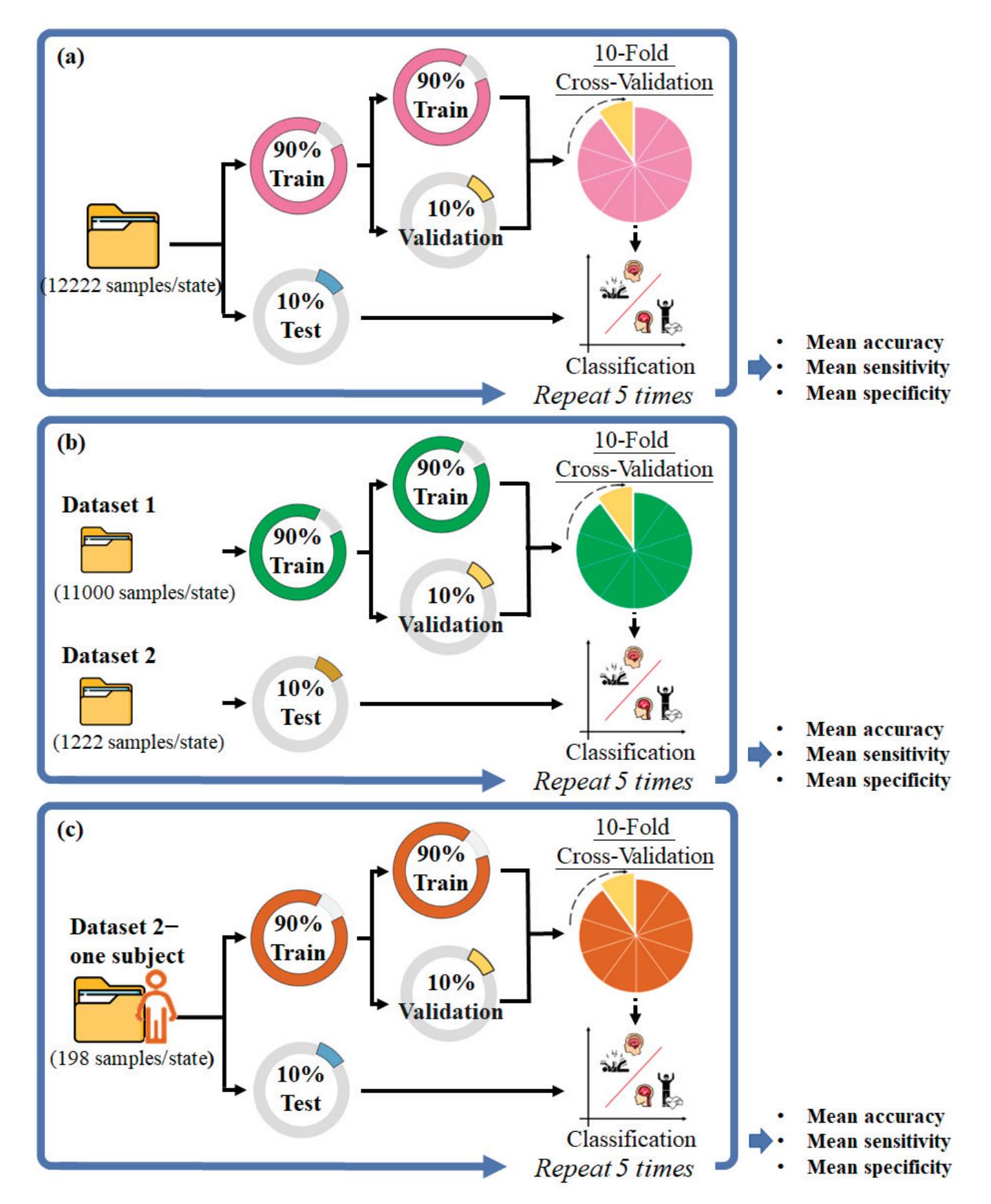
**Figure 2.** Scheme of the training process for a 10-fold cross-validation by using (**a**) recordwise, (**b**) subjectwise, and (**c**) patient-specific approaches.
### 2.2. Experiment 2
#### 2.2.1. Datasets
We used EEG data downloaded from the Sleep Cassette subset of the Sleep-EDFX database [16,21], which consists of 153 polysomnographic (PSG) recordings. Seventy-eight healthy subjects (age = 58.8 ± 22.4 years) were included and the record duration was approximately 20 h, including the whole sleep period. The ECG data were downloaded from the Haaglanden Medisch Centrum (HMC) sleep staging database [16,22], which consists of 154 PSG files. A total of 154 patients with different sleep disorders (age = 53.8 ± 15.4 years) were included, and the record duration was 7–13 h.
205
*Sensors* **2023**, *23*, 2458
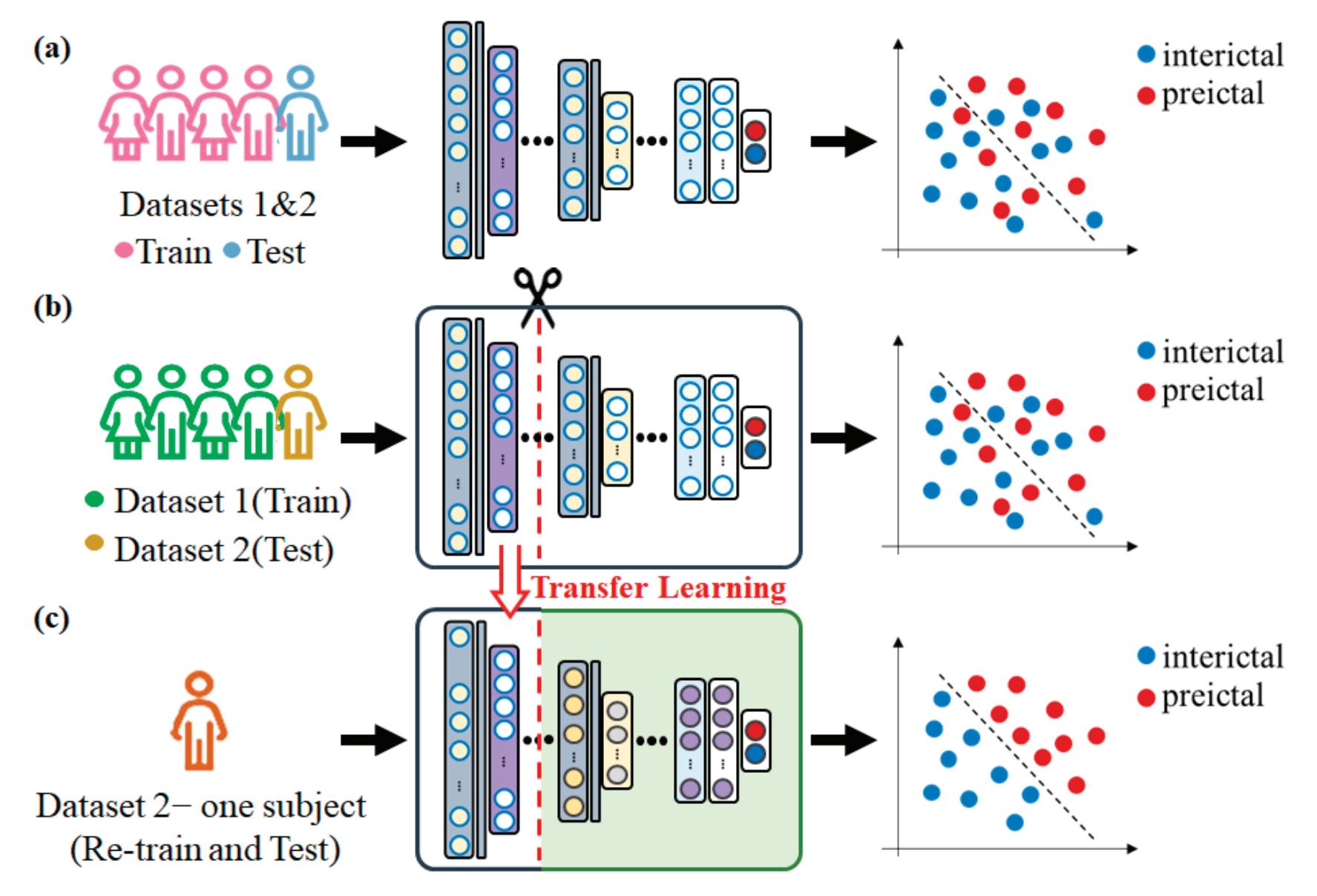
**Figure 3.** Basic procedure for the classification of preictal and interictal periods by using (**a**) recordwise, (**b**) subjectwise, and (**c**) patient-specific approaches.
#### 2.2.2. Data Acquisition
EEG signals were recorded using a dual-channel (Fpz-Cz) cassette recorder at a sampling rate of 100 Hz. Each 30-s epoch was manually labeled by experts in accordance with the R&K standard [23] as belonging to one of six sleep stages: wake, S1, S2, S3, S4, or REM. We coded S1 as NREM1, S2 as NREM2, and combined S3 and S4 as NREM3 in accordance with the American Academy of Sleep Medicine (AASM) standard. ECG signals were recorded using a SOMNOscreen PSG recorder at a sampling frequency of 256 Hz. Each 30-s epoch was manually labeled by sleep technicians at HMC in accordance with the AASM standard (Figure 4).
#### 2.2.3. Data Analysis
EEG signals were preprocessed in two steps using MATLAB R2019a v9.6.0. First, all signals were detrended to remove means, offsets, and slow linear drifts over the time course. These detrended signals were then filtered using a 30-Hz lowpass filter. After preprocessing, the signals were truncated using 30-s windows with 22.5-s overlaps and categorized by sleep state. A total of 16,000 samples were obtained for each state. ECG signals were similarly preprocessed in two steps using MATLAB R2019a v9.6.0. All signals were first detrended to remove means, offsets, and slow linear drifts over the time course. These detrended signals were then filtered using a 0.5–40-Hz bandpass filter. After preprocessing, the truncation process was performed for the EEG signals. A total of 16,000 samples were obtained for each state.
206
*Sensors* **2023**, *23*, 2458
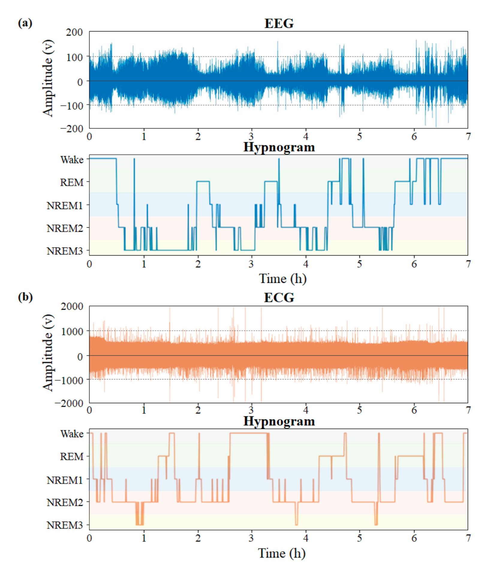
**Figure 4.** Examples of sleep recordings and hypnograms from the (**a**) EEG, and (**b**) ECG datasets.
### 2.2.4. Classification and Performance Evaluation
The CNN model was implemented using Python v3.5.4 running on a personal computer with an Intel Core i7-9700K CPU, NVIDIA Geforce RTX 2060, and 64.0 GB of RAM and running Windows 10 with CUDA 10.1. We modified the model of Jadhav and Mukhopadhyay [24]; the model comprised three blocks and two FC layers. Block\_1 and block\_2 each comprised two convolutional layers, two batch normalipyzation (BN) layers, and one pooling layer; block\_3 comprised one convolutional layer, one BN layer, and one global pooling layer (Table 2). The EEG to ECG transfer learning was performed in three steps: (1) the construction of an EEG-based sleep stage model; (2) transfer of the trained EEG
207
*Sensors* **2023**, *23*, 2458
model to an ECG model; and (3) freezing of block\_1–3, block\_1–2, or block\_1 (i.e., fixing the pretrained weights) and retraining of the unfrozen layers (Figure 5).
**Table 2.** Parameters of the CNN model for sleep staging.
| Block | Layer | Type | Filter Size | # Filter | Stride | Output |
|---------|--------------------------|----------------------|-------------|----------|--------|-----------|
| Block_1 | conv1d_1 | Conv1D | 5 | 16 | 1 | 2996 × 16 |
| | batch normalization_1 | Batch Normalization | - | - | - | 2996 × 16 |
| | conv1d_2 | Conv1D | 5 | 16 | 1 | 2994 × 16 |
| | batch normalization_2 | Batch Normalization | - | - | - | 2994 × 16 |
| | average_pooling1d_1 | AveragePooling1D | 2 | 1 | 2 | 1496 × 16 |
| Block_2 | conv1d_3 | Conv1D | 5 | 32 | 1 | 1492 × 32 |
| | batch normalization_3 | Batch Normalization | - | - | - | 1492 × 32 |
| | conv1d_4 | Conv1D | 5 | 32 | 1 | 1488 × 32 |
| | batch normalization_4 | Batch Normalization | - | - | - | 1488 × 32 |
| | average_pooling1d_2 | AveragePooling1D | 2 | 1 | 2 | 744 × 32 |
| Block_3 | conv1d_5 | Conv1D | 5 | 32 | 1 | 740 × 32 |
| | batch normalization_5 | Batch Normalization | - | - | - | 740 × 32 |
| | global_average_pooling1d | GlobalAveragepooling | - | - | - | 32 |
| | dense_1 | Dense | - | - | - | 32 |
| | dense_2 | Dense | - | - | - | 5 |
Hyperparameters: optimizer = Adam, batch size = 128, learning rate = 0.001 (reduce\_lr: min\_lr = 0.0001).
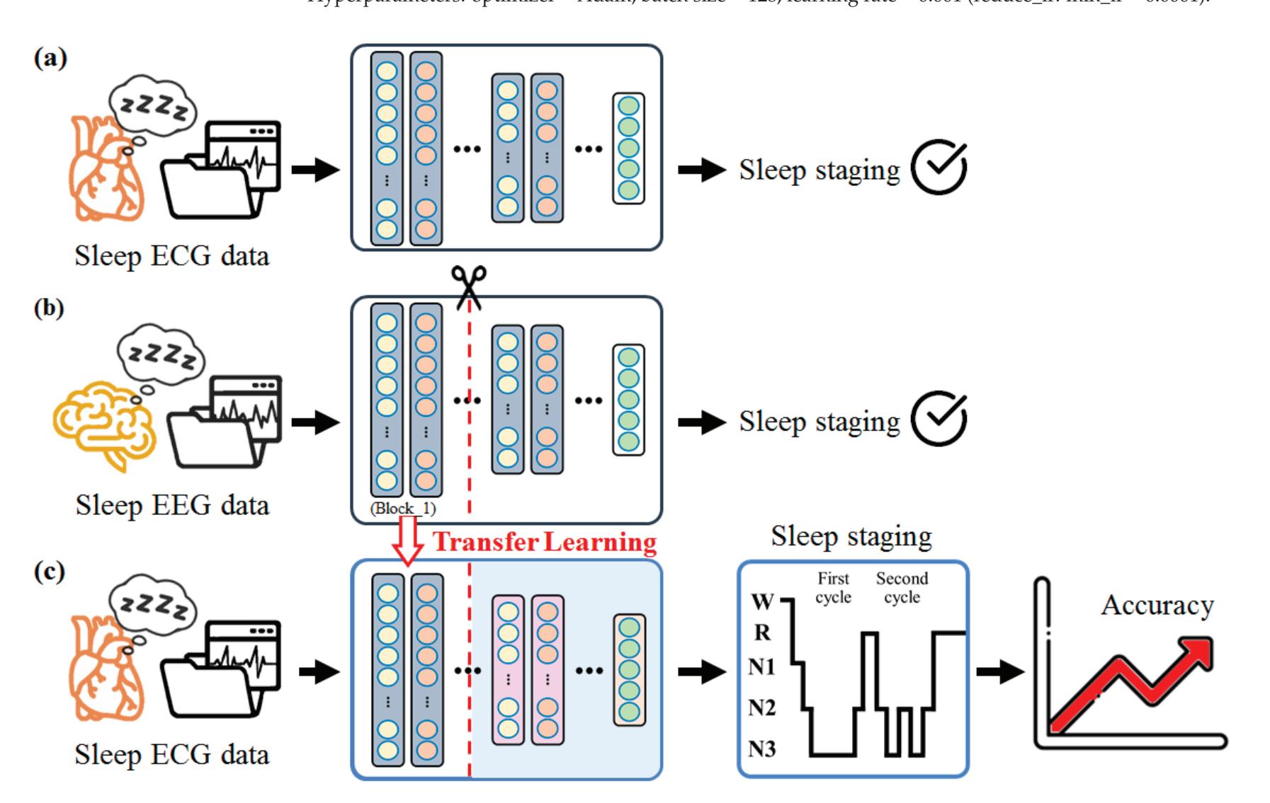
**Figure 5.** Basic procedure for the sleep staging classification in the (**a**) ECG model, (**b**) EEG model, and (**c**) EEG–ECG transfer learning model.
Data were randomly divided into two sets: 80% for training and 20% for testing. A five-fold cross validation was used to evaluate the trained models. The optimal model was then tested using the testing dataset and evaluated its accuracy, Cohen's kappa, and the F1-score. These processes were performed 10 times (Figure 6).
208
*Sensors* **2023**, *23*, 2458
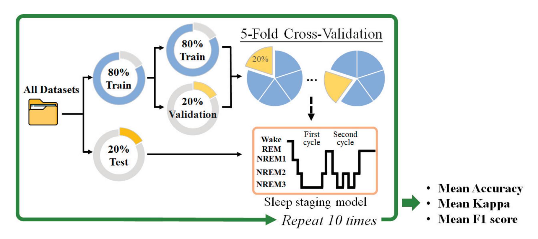
**Figure 6.** Scheme of the training process for a 5-fold cross-validation.
## 3. Results
### 3.1. Experiment 1
The effectiveness of the three training approaches for establishing a CNN-based epilepsy prediction model was investigated. The results for the recordwise training (Table 1) revealed that the accuracy, sensitivity, and specificity for classifying interictal and preictal 20–10-, 30–20-, and 40–30-min states were all greater than 99%, 98%, and 99%, respectively; the training time for all three models was approximately 2 h. Hence, this training approach had an excellent performance, but the training was somewhat time-consuming.
The results for subjectwise training (Table 3) revealed that the accuracy, sensitivity, and specificity for the classifying of interictal and preictal 20–10-, 30–20-, and 40–30-min states were all greater than 82%, 84%, and 83%, respectively; however, the training time for all three models was still approximately 2 h. Hence, a comparison of the results for recordwise and subjectwise training revealed that if the novel subject data were not used for the model training, the test accuracy, sensitivity, and specificity decreased but the training time remained constant.
| Record-Wise Training | | | | |
|-----------------------|----------------|-----------------|-----------------|-----------------|
| | Accuracy (%) | Sensitivity (%) | Specificity (%) | Time |
| preictal 20–10 | 99.37 (±0.14%) | 99.47 (±0.24%) | 99.27 (±0.47%) | 2 h 12 min 43 s |
| preictal 30–20 | 98.61 (±0.20%) | 98.21 (±0.12%) | 99.03 (±0.35%) | 2 h 13 min 43 s |
| preictal 40–30 | 99.59 (±0.22%) | 99.77 (±0.13%) | 99.40 (±0.44%) | 2 h 04 min 06 s |
| Subject-Wise Training | | | | |
| | Accuracy (%) | Sensitivity (%) | Specificity (%) | Time |
| preictal 20–10 | 84.25 (±0.20%) | 82.45 (±1.39%) | 82.45 (±1.39%) | 2 h 17 min 07 s |
| preictal 30–20 | 84.46 (±0.20%) | 84.81 (±0.94%) | 84.12 (±1.09%) | 2 h 19 min 11 s |
| preictal 40–30 | 86.17 (±0.84%) | 88.73 (±0.90%) | 83.60 (±2.05%) | 2 h 20 min 03 s |
The results for patient-specific transfer learning (Table 4) differed from those for recordwise and subjectwise training. The models with 12 frozen layers that were used to classify interictal and preictal 20–10-, 30–20-, and 40–30-min states achieved metrics greater than 90%, 88%, and 95%, respectively, with training times of approximately 2 min. Models with nine frozen layers classifying interictal and preictal 20–10-, 30–20-, and 40–30-min states achieved metrics of 100%, >98%, and >96%, respectively, with training times of 209
*Sensors* **2023**, *23*, 2458
approximately 45 s. Those with six frozen layers achieved metrics of 100%, >97%, and >99% with training times of approximately 40 s, and those with three frozen layers achieved metrics of >96%, >94%, and >98% with training times of approximately 50 s, respectively. In summary, transfer learning training could be completed in approximately 1 min, and the accuracy, sensitivity, and specificity for most patients was high.
**Table 4.** Classification of accuracy, sensitivity, and specificity (mean values) of the patient-specific interictal and preictal classification transfer learning models.
| NO. | # of
Frozen
Layers | Preictal 20–10 | | | | Preictal 30–20 | | | | Preictal 40–30 | | | |
|-----|--------------------------|----------------|------------|------------|-------------|----------------|------------|------------|-------------|----------------|------------|------------|-------------|
| | | Acc
(%) | Sen
(%) | Spe
(%) | Time
(s) | Acc
(%) | Sen
(%) | Spe
(%) | Time
(s) | Acc
(%) | Sen
(%) | Spe
(%) | Time
(s) |
| 2 | 3 | 98.0 | 96.1 | 100 | 42 | 100 | 100 | 100 | 39 | 99.5 | 100 | 99.1 | 43 |
| | 6 | 100 | 100 | 100 | 40 | 100 | 100 | 100 | 37 | 100 | 100 | 100 | 37 |
| | 9 | 100 | 100 | 100 | 35 | 100 | 100 | 100 | 46 | 100 | 100 | 100 | 35 |
| | 12 | 97.5 | 100 | 94.7 | 104 | 97.0 | 93.3 | 100 | 112 | 100 | 100 | 100 | 107 |
| 4 | 3 | 100 | 100 | 100 | 42 | 100 | 100 | 100 | 41 | 100 | 100 | 100 | 43 |
| | 6 | 100 | 100 | 100 | 37 | 100 | 100 | 100 | 37 | 100 | 100 | 100 | 35 |
| | 9 | 100 | 100 | 100 | 35 | 100 | 100 | 100 | 46 | 100 | 100 | 100 | 33 |
| | 12 | 94.9 | 90.4 | 100 | 107 | 100 | 100 | 100 | 118 | 97.5 | 100 | 95.4 | 109 |
| 5 | 3 | 100 | 100 | 100 | 39 | 100 | 100 | 100 | 37 | 100 | 100 | 100 | 33 |
| | 6 | 100 | 100 | 100 | 34 | 100 | 100 | 100 | 34 | 100 | 100 | 100 | 31 |
| | 9 | 100 | 100 | 100 | 43 | 100 | 100 | 100 | 30 | 100 | 100 | 100 | 28 |
| | 12 | 100 | 100 | 100 | 107 | 100 | 100 | 100 | 109 | 100 | 100 | 100 | 103 |
| 7 | 3 | 100 | 100 | 100 | 39 | 100 | 100 | 100 | 36 | 100 | 100 | 100 | 42 |
| | 6 | 100 | 100 | 100 | 36 | 100 | 100 | 100 | 32 | 100 | 100 | 100 | 35 |
| | 9 | 100 | 100 | 100 | 44 | 100 | 100 | 100 | 33 | 100 | 100 | 100 | 32 |
| | 12 | 100 | 100 | 100 | 109 | 100 | 100 | 100 | 109 | 100 | 100 | 100 | 109 |
| 8 | 3 | 100 | 100 | 100 | 41 | 100 | 100 | 100 | 56 | 100 | 100 | 100 | 37 |
| | 6 | 100 | 100 | 100 | 32 | 100 | 100 | 100 | 33 | 100 | 100 | 100 | 36 |
| | 9 | 100 | 100 | 100 | 28 | 100 | 100 | 100 | 29 | 100 | 100 | 100 | 36 |
| | 12 | 100 | 100 | 100 | 109 | 100 | 100 | 100 | 109 | 99.5 | 100 | 97.7 | 109 |
| 9 | 3 | 100 | 100 | 100 | 35 | 99.5 | 100 | 99.33 | 37 | 100 | 100 | 100 | 49 |
| | 6 | 100 | 100 | 100 | 37 | 100 | 100 | 100 | 35 | 100 | 100 | 100 | 35 |
| | 9 | 100 | 100 | 100 | 33 | 100 | 100 | 100 | 34 | 100 | 100 | 100 | 31 |
| | 12 | 100 | 100 | 100 | 108 | 97.5 | 100 | 96.66 | 100 | 100 | 100 | 100 | 109 |
| 10 | 3 | 100 | 100 | 100 | 46 | 100 | 100 | 100 | 44 | 100 | 100 | 100 | 46 |
| | 6 | 100 | 100 | 100 | 34 | 100 | 100 | 100 | 40 | 100 | 100 | 100 | 36 |
| | 9 | 100 | 100 | 100 | 33 | 100 | 100 | 100 | 33 | 100 | 100 | 100 | 32 |
| | 12 | 97.5 | 94.7 | 100 | 89 | 100 | 100 | 100 | 109 | 100 | 100 | 100 | 109 |
| 11 | 3 | 100 | 100 | 100 | 40 | 97.5 | 94.11 | 100 | 41 | 99.5 | 100 | 98.57 | 36 |
| | 6 | 100 | 100 | 100 | 31 | 99 | 97.64 | 100 | 38 | 99.5 | 99.23 | 100 | 33 |
| | 9 | 100 | 100 | 100 | 30 | 98.99 | 100 | 98.6 | 33 | 97.5 | 96.15 | 100 | 29 |
| | 12 | 100 | 100 | 100 | 109 | 94.99 | 88.23 | 100 | 109 | 97.5 | 96.1 | 100 | 109 |
| 13 | 3 | 100 | 100 | 100 | 48 | 98 | 95.7 | 100 | 36 | 100 | 100 | 100 | 34 |
| | 6 | 100 | 100 | 100 | 36 | 99.9 | 98.9 | 100 | 28 | 100 | 100 | 100 | 36 |
| | 9 | 100 | 100 | 100 | 30 | 100 | 100 | 100 | 28 | 100 | 100 | 100 | 29 |
| | 12 | 100 | 100 | 100 | 109 | 100 | 100 | 100 | 105 | 100 | 100 | 100 | 106 |
Specifically, the training time was shortest (~30 s) when freezing nine layers for the classification of interictal and preictal 40–30-min states for nine patients; freezing six layers resulted in the highest accuracy (except for patient 11 with 99.5%). Freezing 12 layers led to the longest training time (~2 min) and the lowest accuracy—which was even lower than when using the recordwise approach. The results thus indicated that transfer learning was superior to recordwise or subjectwise learning.
210
*Sensors* **2023**, *23*, 2458
### 3.2. Experiment 2
Three CNN-based sleep staging models were established: the EEG model, the ECG model, and the EEG–ECG transfer learning model (Table 5). The EEG model for sleep stage classification achieved accuracy, Cohen's kappa, and F1 scores of 92.67%, 0.908, and 92.69%, respectively; the training time (including five-fold cross validation) was approximately 1.5 h; the favorable Cohen's kappa and F1 scores indicated that the model had favorable validity and reliability. The ECG model achieved accuracy, Cohen's kappa, and F1 scores of 86.13%, 0.827, and 86.07%, respectively; the training time was still approximately 1.5 h. Finally, the EEG–ECG transfer learning model with block\_1 frozen achieved metrics superior to the ECG-only model: 88.64%, 0.858, and 88.59%, with a lower training time of approximately 47 min. Freezing block\_1 and block\_2 or all three blocks resulted in lower scores than the ECG model; however, the training time was far shorter than that for the ECG model at approximately 17 min. Hence, the model with block\_1 frozen (two convolutional layers, two BN layers, and one pooling layer) achieved both a higher performance and a lower training time than the ECG-only model.
**Table 5.** Classification accuracy, Cohen's kappa, and F1 score (mean ± standard deviation) of the EEG model, ECG model, and the EEG–ECG transfer learning model.
| Model | Accuracy | Kappa | F1 | Time |
|----------------------------|----------------|----------------|----------------|-----------------|
| EEG | 92.67 (±0.45%) | 0.908 (±0.006) | 92.69 (±0.45%) | 1 h 32 min 42 s |
| ECG | 86.13 (±1.49%) | 0.827 (±0.019) | 86.07 (±1.46%) | 1 h 38 min 10 s |
| EEG-ECG (frozen block_1) | 88.64 (±1.00%) | 0.858 (±0.013) | 88.59 (±1.01%) | 47 min 31 s |
| EEG-ECG (frozen block_1&2) | 82.16 (±0.56%) | 0.777 (±0.007) | 82.12 (±0.52%) | 17 min 00 s |
| EEG-ECG (frozen block_1~3) | 63.38 (±0.62%) | 0.542 (±0.008) | 63.19 (±0.60%) | 17 min 05 s |
Figure 7 illustrates the accuracy and loss functions of the EEG, ECG, and EEG–ECG models. An early stop strategy with a patience of 10 was implemented to terminate the training process. The validation accuracy and loss curve of the EEG model increased and decreased quickly, respectively. The validation accuracy and loss curves of the ECG model both fluctuated initially and then stabilized. For the EEG–ECG transfer learning model, the validation accuracy and loss curve were initially high and low, respectively, but slowly stabilized after fluctuating slightly. Overall, overfitting was not evident for any of the three models; hence, the training was judged to be effective.
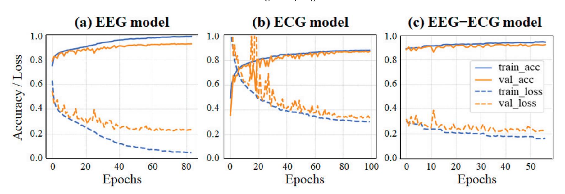
**Figure 7.** Accuracy (upper panel) and loss (lower panel) functions of the (**a**) EEG model, (**b**) ECG model, and (**c**) EEG–ECG model (frozen block\_1).
Figure 8 presents the confusion matrixes for the three sleep staging models. Except for NREM1, which was frequently misclassified as waking or NREM2, high classification accuracies were achieved. Hence, the three models achieved favorable classification results and no substantial imbalance was identified.
211
*Sensors* **2023**, *23*, 2458
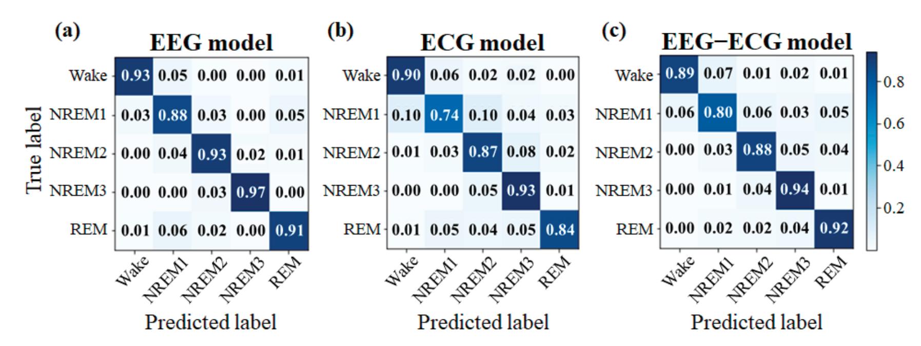
**Figure 8.** Confusion matrix of the (**a**) EEG, (**b**) ECG, and (**c**) EEG–ECG model (frozen block\_1).
## 4. Discussion
### 4.1. Experiment 1
Recordwise training is a commonly used approach in initial deep-learning research. In training, data from all subjects in a database are randomly divided into a training set and testing set; each sample (from the same subject) is considered independent. For example, Acharya et al. [25] developed a computer-aided seizure diagnosis system to automatically distinguish the class of EEG signals (i.e., normal, preictal, or seizure) by using a 13-layer CNN model. They employed a dataset of 100 epochs for each of five healthy subjects and five patients with epilepsy, while 90% of the total data was set for training. Their model achieved an accuracy, specificity, and sensitivity of 88.67%, 90.00%, and 95.00%, respectively. Moreover, Wei et al. [26] proposed a long-term recurrent CNN for discriminating preictal from interictal states for seizure prediction. They similarly used a 9:1 ratio to divide the EEG data of each subject into training and test sets. Their seizure prediction model achieved an accuracy of 93.40%, prediction sensitivity of 91.88%, and specificity of 86.13%. In our experiment, all EEG samples from 27 patients with epilepsy in two datasets were mixed and were randomly divided into training and test sets (1222 samples per state). The classification accuracy, sensitivity, and specificity for interictal and preictal (regardless of period) states were all greater than 98%. These results indicate that the recordwise trained model is often only effective for classifying the used dataset, and its performance on novel data is poor [7].
Many studies have adopted subjectwise training for deep-learning models in which data from an individual are included in either the training or the testing set. This method better matches practical applications of the trained model to novel patients. However, the accuracy is an inevitable issue. In our experiment, we used EEG data from one dataset (Siena Scalp EEG database) for training, and EEG data from another dataset (Zenodo database) for testing. The accuracy decreased from 98% for the recordwise approach to only 84%; this may be attributable to the inter-person differences and the diversity of the data. This problem of a cross-subject domain shift has partly been addressed by some scholars. For example, Wang et al. [27] proposed a multiscale CNN, known as SEEG-Net, for evaluating drug-resistant epilepsy. They conducted cross-validation on a multicenter stereoelectroencephalography dataset by using the leave-one-group-out method and achieved an accuracy of 94.12% and 87.02% for the MAYO and FNUSA datasets, respectively; leave-one-subject-out cross validation on a private clinical dataset led to an accuracy of 93.85%. Although their proposed model performed highly in detecting pathological activity, it still has insufficient generalizability for practical applications.
The quality of EEG signals is affected by breathing, blinking, and swallowing during the measurement. In addition, individual differences may also affect evaluations based on these signals [28]. To avoid overfitting, deep-learning requires an enormous volume 212
*Sensors* **2023**, *23*, 2458
of training data and hence a long training time, delaying system development. Hence, we selected patient-specific transfer learning for retraining our model; specifically, data for a specific subject in the Zenodo dataset were used to fine-tune a model pretrained on the Siena Scalp EEG database. This method required a smaller amount of data, achieved high accuracy, and required little additional training time to produce the customized model. Layer-wise transfer learning is a commonly used approach in which some layers are frozen to decrease the training time. If a few layers are frozen, the model has high elasticity but requires a longer training time; by contrast, freezing many layers reduces the training time but often reduces the accuracy. Our experimental results indicated that a model with six frozen layers had a short training time (~40 s) and achieved the highest accuracy of nearly 100%. Freezing nine layers achieved a similar performance to freezing six layers; however, the imperfect results for patient 11 revealed that such a model may have insufficient elasticity to be applicable to all individuals. The optimal number of frozen layers may depend on the size of the training data [29]. Hence, for smaller datasets, training the FC layers alone is insufficient; some convolutional layers must also be trained to obtain a stable, accurate model.
Finally, we compared the accuracy rates of our model with those of models reported by other recent studies on epileptic seizure prediction using EEG data (Table 6). Dissanayake et al. [30] extracted Mel-frequency cepstrum coefficients (MFCCs) features from EEG signals and used them in a graph neural network (C-GNN) based on geometric deep-learning to predict epileptic seizures. Their subject-independent models were trained through a 10-fold cross-validation with over a 95% accuracy in both CHB-MIT and Siena databases. Zhao et al. [31] proposed a novel end-to-end model AddNet-SCL for seizure prediction based on EEG signals. They used a quasi-patient-specific method (i.e., 0.75 × (1−1/N), 0.25 × (1−1/N), and 1/N of a patient's EEG data were used for the training, validation, and testing, respectively; where N was the number of seizure events) to conduct separate model training for each subject from CHB-MIT and Kaggle databases, and achieved 0.94 AUC and 0.831 AUC, respectively. Considering the robustness and generalization of the learning models, either training manner, i.e., subject independent or patient-specific, could achieve a high performance, while ours had the highest accuracy, specificity, and sensitivity. Furthermore, the use of raw EEG data in our experiment can facilitate the processes of data collection and processing and benefit future applications, bypassing the need for feature extraction or selection.
**Table 6.** Performance of different seizure prediction systems based on CNNs with EEG signals.
| Study | Dataset | Input | Model | Training
Type | Acc
(%) | Sen
(%) | Spe
(%) |
|-------------------------|--------------------------|-------------------|----------------------------------|------------------|------------|------------|------------|
| Dissanayake et al. [30] | Siena EEG | MFCCs | C-GNN
(distance-based) | S-Ind | 96.0 | 96.0 | 96.6 |
| | | | C-GNN
(partially learned) | | 95.5 | 95.1 | 95.1 |
| Zhao et al. [31] | CHB-MIT | Raw data | 1D-CNN | P-Spc | - | 88.7 | - |
| | | | ResCNN | | | 89.9 | |
| | | | SCL-AddNets | | | 93 | |
| This Study | CHB-MIT | Raw data
(GFP) | 1D-CNN
+
transfer learning | P-Spc | 99.73 | 99.79 | 99.65 |
| | Siena EEG
+
Zenodo | Raw data
(GFP) | 1D-CNN
+
transfer learning | P-Spc | 99.9 | 99.9 | 100 |
S-Ind: subject independent; P-Spc: patient-specific.
### 4.2. Experiment 2
Silveira et al. [32] used random forest to classify 106,376 single-channel EEG epochs from the Physionet public database into two- to six-state sleep stages. They computed 213
*Sensors* **2023**, *23*, 2458
the kurtosis, skewness, and variance of the coefficients decomposed through the discrete wavelet transform as classification features. The accuracy and Cohen's kappa were >90% and >0.8, respectively, demonstrating that single-channel EEG is a feasible method of sleep staging. More recently, many studies have applied various deep-learning models for sleep staging with the goal of achieving automatic and accurate classification by avoiding manual feature extraction. For example, Yildirim et al. [33] developed a 1D-CNN model by using EEG signals from two public databases (Sleep-EDF and Sleep-EDFX) for the sleep stage classification. The accuracy of the model for five sleep classes on single-channel EEGs from the Sleep-EDF and the Sleep-EDFX databases was 90.83% and 90.48%, respectively. In our experiment, we also used the Fpz-Cz single-channel EEG signals from the Sleep-EDFX database for five-class sleep staging to train a modified 1D-CNN (10 layers in total; 9 layers fewer than in the model of [33]). The accuracy reached 92.67%, indicating that using fewer convolutional layers and max pooling instead of average pooling can slightly improve both the accuracy (~2%) and training efficiency. Although max pooling retains key sleep features in EEG, it ignores secondary features that may be effective for classification. By contrast, average pooling retains these features.
Due to the increasing prevalence of wearable biosignal sensors, many researchers have begun to study ECG sleep staging as an alternative to EEG staging. For example, Ebrahimi et al. [34] extracted features from ECG-derived respiration signals based on the R and S waves of the QRS complex, raw thoracic respiratory rate (R), and heart rate variability (HRV) and evaluated the performance of various signal combinations in an SVM automatic sleep staging model. Their best accuracy (89.32%) for classifying four stages—wake, Stage 2, slow wave sleep, and REM—was obtained when using HRV and R signals. Furthermore, Wei et al. [35] extracted 25 features from HRV and R signals and used LSTM for the two- to five-class sleep staging of patients with mental disorders, achieving accuracies of 89.84%, 84.07%, 77.76%, and 71.16% and Cohen's kappa of 0.52, 0.58, 0.55, and 0.52, respectively, for the four classification tasks. These results indicate that increasing the number of classes decreases the performance; improving the accuracy requires the combination of various signals with different features. However, manual feature selection is time-consuming. Hence, some researchers have used deep-learning models for ECG sleep staging. For example, Tang et al. [36] used a CNN with gated recurrent units to classify sleep stages into four classes on the basis of single-lead ECG signals from the three public datasets SHHS2, SHHS1, and MESA. Their best accuracy and Cohen's kappa were 80.6% and 0.70, respectively—a substantial improvement over previous attempts at cross-dataset classification. In our experiment, we used a CNN model for five-class sleep staging and an achieved average accuracy was 86.13%, which demonstrates that the model structure is effective for both EEG and ECG signals; the model achieved favorable performance for both signals, but the ECG model required more computational resources and training time.
Therefore, we applied transfer learning to improve the performance of the ECG model by basing it on the highly accurate EEG model. Freezing block\_1 produced an EEG–ECG transfer learning model with an accuracy of 88.64%, a small improvement (~2.5%) compared with the ECG-only model. Radha et al. [37] trained an LSTM model to classify four-class sleep stages by using ECG data (292 participants, 584 recordings) and then transferred some of its weights to photoplethysmography (PPG) data (60 participants, 101 recordings) by using three transfer-learning strategies. The accuracy and Cohen's kappa of the ECG–PPG model were 76.36% and 0.65, respectively—a substantial improvement over those of the PPG model (69.82% and 0.55). This result demonstrates the merit of transfer learning if similar data are reused. However, few studies have attempted cross-signal transfer learning. Phan et al. [10] trained two recurrent neural networks in the source domain (a large database; the Montreal Archive of Sleep Studies database in this case) and then finetuned them in the target domain (two small databases: the SurreycEEGrid database and the Sleep Cassette and the Sleep Telemetry subsets of the Sleep-EDFX database). The transfer learning achieved an improvement in accuracy of 1.5% for their SeqSleepNet+ network (78.5% for EEG-only to 80.0% for EEG-EOG) and 3.5% for their DeepSleepNet+ network
214
*Sensors* **2023**, *23*, 2458
(75.9% to 79.4%). These transfer-learning studies reveal that the knowledge transfer from the same or similar signals can considerably increase model performance; for different signals, however, it does not greatly increase the accuracy but substantially reduces the training time, in our case. Moreover, if too many layers are frozen (too much knowledge is shared), training the new model has a limited effect and the model may fit the data poorly, resulting in high-speed training but low performance.
Finally, we compared the accuracy rates of our model with those of models reported by other recent studies on sleep staging using EEG data (Table 7). Li et al. [38] proposed an EEGSNet model based on CNN and bi-directional LSTM (Bi-LSTM) to extract features from the EEG spectrogram and classify them into five sleep stages. They trained their model using a 20-fold or leave-one-out cross-validation according to the size of the datasets. The accuracies were 94.17%, 86.82%, 83.02%, and 85.12%, respectively, for the sleep-edfx-8, sleep-edfx-20, sleep-edfx-78, and SHHS datasets. Jadhav et al. [24] evaluated the raw EEG epochs, short-time Fourier transform (STFT), and stationary wavelet transform (SWT) in the same dataset (i.e., sleep-edfx-78) by using CNN models. Their subject-wise models were trained through a 20-fold cross-validation with over 83% accuracy. For the classification of five sleep stages, our model with fewer layers achieved a better performance and the direct use of raw EEG data in our experiment can be of benefit for fast diagnosis. Table 8 shows the comparison of our model with other recent closely related studies using ECG data. Urtnasan et al. [8] used a deep convolutional recurrent (DCR) model based on the CNN and a gated recurrent unit (GRU) for the automatic scoring of sleep stages. They trained and tested the model using the ECG signals of 89 subjects and 23 subjects, respectively, randomly selected from the dataset and achieved an overall accuracy of 74.2% for five classes and 86.4% for three classes. Tang et al. [36] pre-trained a model built on five CNN blocks, bi-directional GRU layers, and a fully connected layer with a dataset and then re-trained it with another dataset with an improvement of 20%. Considering the resources and time, they randomly sampled 100 subjects (70% for training and 30% for testing) from each dataset. There is still room for improvement in the effect of using ECG signals alone for classification. By using transfer learning from EEG to ECG, our model could classify more classes with a better performance, which demonstrates the feasibility of automatic sleep staging using ECG signals.
**Table 7.** Performance of different sleep staging systems based on CNNs with EEG signals.
| Study | Dataset | Input | Model | # CNN Layer | Sleep Stage | Acc (%) | Kappa | F1 (%) |
|--------------------|------------|-------------------------|----------------------------|-------------|-------------------|-------------------------|-------------------------|-------------------------|
| Li et al. [38] | sleep-edfx | Spectrogram | EEGSNet | 15 | Wake-REM-N1-N2-N3 | 83.02 | 0.770 | 77.26 |
| Jadhav et al. [24] | sleep-edfx | Raw data
SWT
STFT | 1D-CNN
2D-CNN
2D-CNN | 6
6
4 | Wake-REM-N1-N2-N3 | 83.59
85.49
85.81 | 0.780
0.800
0.800 | 77.00
78.70
79.70 |
| This Study | sleep-edfx | Raw data | 1D-CNN | 5 | Wake-REM-N1-N2-N3 | 92.67 | 0.908 | 92.69 |
**Table 8.** Performance of different sleep staging systems based on CNNs with ECG signals.
| Study | Dataset | Input | Model | # Class | Sleep Stages | Acc (%) | Kappa | F1 (%) |
|---------------------|---------------------------|----------|----------------------------------|---------|------------------------------------|-------------------------|-------------------------|----------------|
| Urtnasan et al. [8] | Samsung
Medical Center | Raw data | CNN+GRU | 3
5 | Wake-NREM-REM
Wake-REM-N1-N2-N3 | 86.40
74.20 | -
- | -
- |
| Tang et al. [36] | SHHS2
SHHS1
MESA | Raw data | CNN+GRU
(Domain adaptation) | 4 | Wake-REM
Light-Deep | 78.70
74.80
80.60 | 0.749
0.675
0.705 | -
-
- |
| This Study | HMC sleep
center | Raw data | 1D-CNN (ECG)
1D-CNN (EEG-ECG) | 5 | Wake-REM-N1-N2-N3 | 86.13
88.64 | 0.827
0.858 | 86.07
88.59 |
Our experiments have some limitations. First, the sample size was insufficient. Including more databases in the training and test sets would improve the reliability of the model. 215
*Sensors* **2023**, *23*, 2458
Second, temporal information was not considered. Automatic feature extraction coupled with time series training, such as CNN-LSTM, may be more effective.
## 5. Conclusions
This study attempted to apply cross-domain transfer learning for two EEG-based classification tasks—seizure prediction and sleep staging—to explore its effects on recognition performance.
In Experiment 1, binary classification models were trained using a recordwise approach to test the architecture of our model; this model achieved an accuracy, specificity, and sensitivity of >98%. Subsequent subjectwise training simulated practical applications in which the test and training data were independent; this model achieved an accuracy, specificity, and sensitivity of >82%. Due to this dramatic decrease in the model performance, cross-dataset transfer learning was used to train patient-specific models; the model with six frozen layers achieved an accuracy, specificity, and sensitivity of 100% for seven out of nine subjects and >97% for the remaining two; moreover, only 40 s of additional training time was required. By applying transfer learning, the model could learn the EEG characteristics of an individual to achieve personalized and accurate detection that could increase the practicality of seizure prediction.
In Experiment 2, transfer learning on different signal sources for five-class sleep staging prediction was attempted. The same modified model architecture was used to build EEG and ECG models. As expected, the accuracy, Cohen's kappa, and F1-score (92.67%, 0.908, and 2.695%) of the EEG model were superior to those of the ECG model (86.13%, 0.827, and 86.07%). However, transfer learning produced an EEG–ECG model with an accuracy approximately 2.5% greater than that of the ECG model. Although this crosssignal transfer-learning method achieved little performance improvement, the training time was reduced by >50% compared with that for the ECG-only model, effectively reducing the computing resource consumption. Additional studies should be conducted regarding the challenges of knowledge transfer between different signals. To the best of our knowledge, this experiment is the first to demonstrate the feasibility of cross-signal transfer learning from EEG to ECG for sleep staging. EEG measurement is inconvenient and uncomfortable; hence, using ECG for sleep staging could enable practical applications, such as wearable devices employed for sleep analysis and recording sleep quality.
In summary, EEG can be used to detect brain abnormalities and provides an effective basis for patient evaluation. However, its limitations restrict its use in practice. Crossdomain transfer learning strategies may be able to overcome these problems for further specific uses, such as precision medicine, portable devices, or rare disease detection, in simple or original model structures.
**Author Contributions:** All authors contributed to the study conception and design. Material preparation, data collection and analysis were performed by P.-C.C. and W.-C.H. The first draft of the manuscript was written by C.-Y.Y. and all authors commented on previous versions of the manuscript. All authors have read and agreed to the published version of the manuscript.
**Funding:** English editing was funded by the National Science and Technology Council (MOST 111-2221-E-130-001-MY3), Taiwan.
**Institutional Review Board Statement:** Not applicable.
**Informed Consent Statement:** Not applicable.
**Data Availability Statement:** The data used in this study are openly available in Siena scalp EEG database at [https://physionet.org/content/siena-scalp-eeg/1.0.0/ accessed on 10 February 2022], Zenodo at [https://zenodo.org/record/1415495 accessed on 10 February 2022], Sleep-EDF expanded database at [https://physionet.org/content/sleep-edfx/1.0.0/ accessed on 10 February 2022], and Haaglanden Medisch Centrum sleep staging database at [https://physionet.org/content/hmc-sleepstaging/1.0.1/ accessed on 10 February 2022].
216
*Sensors* **2023**, *23*, 2458
**Acknowledgments:** This study was supported in part by the National Science and Technology Council (MOST 111-2221-E-130-001-MY3), Taiwan.
**Conflicts of Interest:** The authors declare no conflict of interest.
## References
- 1. Binnie, C.D.; Prior, P.F. Electroencephalography. *J. Neurol. Neurosurg. Psychiatry Res.* **1994**, *57*, 1308–1319. [CrossRef]
- 2. Oh, S.L.; Hagiwara, Y.; Raghavendra, U.; Yuvaraj, R.; Arunkumar, N.; Murugappan, M.; Acharya, U.R. A deep learning approach for Parkinson's disease diagnosis from EEG signals. *Neural. Comput. Appl.* **2018**, *32*, 10927–10933. [CrossRef]
- 3. Rim, B.; Sung, N.J.; Min, S.; Hong, M. Deep learning in physiological signal data: A survey. *Sensors* **2020**, *20*, 969. [CrossRef] [PubMed]
- 4. Han, C.; Peng, F.; Chen, C.; Li, W.; Zhang, X.; Wang, X.; Zhou, W. Research progress of epileptic seizure predictions based on electroencephalogram signals. *J. Biomed. Eng.* **2021**, *38*, 1193–1202. [PubMed]
- 5. Yang, C.Y.; Huang, Y.Z. Parkinson's Disease Classification Using machine learning approaches and resting-state EEG. *J. Med. Biol. Eng.* **2022**, *42*, 263–270. [CrossRef]
- 6. Shoeibi, A.; Sadeghi, D.; Moridian, P.; Ghassemi, N.; Heras, J.; Alizadehsani, R.; Khadem, A.; Kong, Y.; Nahavandi, S.; Zhang, Y.; et al. Automatic diagnosis of schizophrenia in EEG signals using CNN-LSTM models. *Front. Neurosci.* **2021**, *15*, 777977. [CrossRef]
- 7. Cimtay, Y.; Ekmekcioglu, E. Investigating the use of pretrained convolutional neural network on cross-subject and cross-dataset EEG emotion recognition. *Sensors* **2020**, *20*, 2034. [CrossRef]
- 8. Urtnasan, E.; Park, J.U.; Joo, E.Y.; Lee, K.J. Deep convolutional recurrent model for automatic scoring sleep stages based on single-lead ECG signal. *Diagnostics* **2022**, *12*, 1235. [CrossRef]
- 9. Panigrahi, S.; Nanda, A.; Swarnkar, T. A Survey on Transfer Learning. In *Intelligent and Cloud Computing*; Springer: Singapore, 2021; pp. 781–789.
- 10. Phan, H.; Chén, O.Y.; Koch, P.; Lu, Z.; McLoughlin, I.; Mertins, A.; De Vos, M. Towards more accurate automatic sleep staging via deep transfer learning. *IEEE Trans. Biomed. Eng.* **2021**, *68*, 1787–1798. [CrossRef]
- 11. Wan, Z.; Yang, R.; Huang, M.; Zeng, N.; Liu, X. A review on transfer learning in EEG signal analysis. *Neurocomputing* **2021**, *421*, 1–14. [CrossRef]
- 12. Zargar, B.S.; Mollaei, M.R.K.; Ebrahimi, F.; Rasekhi, J. Generalizable epileptic seizures prediction based on deep transfer learning. *Cogn. Neurodyn.* **2023**, *17*, 119–131. [CrossRef] [PubMed]
- 13. Bird, J.J.; Kobylarz, J.; Faria, D.R.; Ekárt, A.; Ribeiro, E.P. Cross-domain MLP and CNN transfer learning for biological signal processing: EEG and EMG. *IEEE Access* **2020**, *8*, 54789–54801. [CrossRef]
- 14. Moshe, S.L.; Perucca, E.; Ryvlin, P.; Tomson, T. Epilepsy: New advances. *Lancet* **2015**, *385*, 884–898. [CrossRef] [PubMed]
- 15. Lun, X.; Yu, Z.; Chen, T.; Wang, F.; Hou, Y. A Simplified CNN Classification Method for MI-EEG via the Electrode Pairs Signals. *Front. Hum. Neurosci.* **2020**, *14*, 338. [CrossRef]
- 16. Goldberger, A.L.; Amaral, L.A.; Glass, L.; Hausdorff, J.M.; Ivanov, P.C.; Mark, R.G.; Mietus, J.E.; Moody, G.B.; Peng, C.K.; Stanley, H.E. PhysioBank, PhysioToolkit, and PhysioNet: Components of a new research resource for complex physiologic signals. *Circulation* **2000**, *101*, 215–220. [CrossRef]
- 17. Detti, P.; Vatti, G.; Zabalo, M.D.L. EEG Synchronization Analysis for seizure prediction: A study on data of noninvasive recordings. *Processes* **2020**, *8*, 846. [CrossRef]
- 18. Billeci, L.; Marino, D.; Insana, L.; Vatti, G.; Varanini, M. Patient-specific seizure prediction based on heart rate variability and recurrence quantification analysis. *PLoS ONE* **2020**, *13*, e0204339. [CrossRef]
- 19. Skrandies, W. Data reduction of multichannel fields: Global field power and principal component analysis. *Brain Topogr.* **1989**, *2*, 73–80. [CrossRef]
- 20. Wang, X.; Wang, X.; Liu, W.; Chang, Z.; Kärkkäinen, T.; Cong, F. One dimensional convolutional neural networks for seizure onset detection using long-term scalp and intracranial EEG. *Neurocomputing* **2021**, *459*, 212–222. [CrossRef]
- 21. Kemp, B.; Zwinderman, A.H.; Tuk, B.; Kamphuisen, H.A.; Oberyé, J.J. Analysis of a sleep-dependent neuronal feedback loop: The slow-wave microcontinuity of the EEG. *IEEE Trans. Biomed. Eng.* **2000**, *47*, 1185–1194. [CrossRef]
- 22. Alvarez-Estevez, D.; Rijsman, R.M. Inter-database validation of a deep learning approach for automatic sleep scoring. *PLoS ONE* **2021**, *16*, e0256111. [CrossRef]
- 23. Hori, T.; Sugita, Y.; Koga, E.; Shirakawa, S.; Inoue, K.; Uchida, S.; Kuwahara, H.; Kousaka, M.; Kobayashi, T.; Tsuji, Y.; et al. Proposed supplements and amendments to 'A Manual of Standardized Terminology, Techniques and Scoring System for Sleep Stages of Human Subjects', the Rechtschaffen & Kales (1968) standard. *Psychiatry Clin.* **2001**, *55*, 305–310.
- 24. Jadhav, P.; Mukhopadhyay, S. Automated Sleep Stage Scoring Using Time-frequency spectra convolution neural network. *IEEE Trans. Instrum. Meas.* **2022**, *71*, 2510309. [CrossRef]
- 25. Acharya, U.R.; Oh, S.L.; Hagiwara, Y.; Tan, J.H.; Adeli, H. Deep convolutional neural network for the automated detection and diagnosis of seizure using EEG signals. *Comput. Biol. Med.* **2018**, *100*, 270–278. [CrossRef]
- 26. Wei, X.; Zhou, L.; Zhang, Z.; Chen, Z.; Zhou, Y. Early prediction of epileptic seizures using a long-term recurrent convolutional network. *J. Neurosci.* **2019**, *327*, 108395. [CrossRef]
217
*Sensors* **2023**, *23*, 2458
- 27. Wang, Y.; Yang, Y.; Cao, G.; Guo, J.; Wei, P.; Feng, T.; Dai, Y.; Huang, J.; Kang, G.; Zhao, G. SEEG-Net: An explainable and deep learning-based cross-subject pathological activity detection method for drug-resistant epilepsy. *Comput. Biol. Med.* **2022**, *148*, 105703. [CrossRef]
- 28. Al-Kadi, M.I.; Reaz, M.B.I.; Ali, M.A.M. Evolution of electroencephalogram signal analysis techniques during anesthesia. *Sensors* **2013**, *13*, 6605–6635. [CrossRef]
- 29. Ardalan, Z.; Subbian, V. Transfer learning approaches for neuroimaging analysis: A scoping review. *Front. Artif. Intell.* **2022**, *5*, 780405. [CrossRef]
- 30. Dissanayake, T.; Fernando, T.; Denman, S.; Sridharan, S.; Fookes, C. Geometric Deep learning for subject independent epileptic seizure prediction using scalp EEG signals. *IEEE J. Biomed. Health Inform.* **2022**, *26*, 527–538. [CrossRef]
- 31. Zhao, Y.; Li, C.; Qian, R.; Song, R.; Chen, X. Patient-specific seizure prediction via adder nNetwork and supervised contrastive learning. *IEEE Trans. Neural. Syst. Rehabil. Eng.* **2022**, *30*, 1536–1547. [CrossRef]
- 32. da Silveira, T.L.; Kozakevicius, A.J.; Rodrigues, C.R. Single-channel EEG sleep stage classification based on a streamlined set of statistical features in wavelet domain. *Med. Biol. Eng. Comput.* **2017**, *5*, 343–352. [CrossRef]
- 33. Yildirim, O.; Baloglu, U.B.; Acharya, U.R. Deep learning model for automated sleep stages classification using PSG signals. *Int. J. Environ. Res. Public Health* **2019**, *16*, 599. [CrossRef] [PubMed]
- 34. Ebrahimi, F.; Setarehdan, S.K.; Nazeran, H. Automatic sleep staging by simultaneous analysis of ECG and respiratory signals in long epochs. *Biomed. Signal. Process. Control* **2015**, *1*, 69–79. [CrossRef]
- 35. Wei, Y.; Qi, X.; Wang, H.; Liu, Z.; Wang, G.; Yan, X. A multi-class automatic sleep staging method based on long short-term memory network using single-lead electrocardiogram signals. *IEEE Access* **2019**, *7*, 85959–85970. [CrossRef]
- 36. Tang, M.; Zhang, Z.; He, Z.; Li, W.; Mou, X.; Du, L.; Wang, P.; Zhao, Z.; Chen, X.; Li, X.; et al. Deep adaptation network for subject-specific sleep stage classification based on a single-lead ECG. *Biomed. Signal. Process. Control* **2022**, *75*, 103548. [CrossRef]
- 37. Radha, M.; Fonseca, P.; Moreau, A.; Ross, M.; Cerny, A.; Anderer, P.; Long, X.; Aarts, R.M. A deep transfer learning approach for wearable sleep stage classification with photoplethysmography. *NPJ Digit. Med.* **2021**, *4*, 135. [CrossRef]
- 38. Li, C.; Qi, Y.; Ding, X.; Zhao, J.; Sang, T.; Lee, M. A deep learning method approach for sleep stage classification with EEG spectrogram. *Int. J. Environ. Res. Public Health* **2022**, *19*, 6322. [CrossRef]
**Disclaimer/Publisher's Note:** The statements, opinions and data contained in all publications are solely those of the individual author(s) and contributor(s) and not of MDPI and/or the editor(s). MDPI and/or the editor(s) disclaim responsibility for any injury to people or property resulting from any ideas, methods, instructions or products referred to in the content.
218


*Article*
# A Sparse Representation Classification Scheme for the Recognition of Affective and Cognitive Brain Processes in Neuromarketing
**Vangelis P. Oikonomou \*, Kostas Georgiadis, Fotis Kalaganis, Spiros Nikolopoulos and Ioannis Kompatsiaris**
Information Technologies Institute, Centre for Research and Technology Hellas, CERTH-ITI, 6th km Charilaou-Thermi Road, 57001 Thessaloniki, Greece
**\*** Correspondence: viknmu@iti.gr
**Abstract:** In this work, we propose a novel framework to recognize the cognitive and affective processes of the brain during neuromarketing-based stimuli using EEG signals. The most crucial component of our approach is the proposed classification algorithm that is based on a sparse representation classification scheme. The basic assumption of our approach is that EEG features from a cognitive or affective process lie on a linear subspace. Hence, a test brain signal can be represented as a linear (or weighted) combination of brain signals from all classes in the training set. The class membership of the brain signals is determined by adopting the Sparse Bayesian Framework with graph-based priors over the weights of linear combination. Furthermore, the classification rule is constructed by using the residuals of linear combination. The experiments on a publicly available neuromarketing EEG dataset demonstrate the usefulness of our approach. For the two classification tasks offered by the employed dataset, namely affective state recognition and cognitive state recognition, the proposed classification scheme manages to achieve a higher classification accuracy compared to the baseline and state-of-the art methods (more than 8% improvement in classification accuracy).
**Keywords:** sparse representation classification; brain computer interfaces; neuromarketing; electroencephalography
**Citation:** Oikonomou, V.P.; Georgiadis, K.; Kalaganis, F.; Nikolopoulos, S.; Kompatsiaris, I. A Sparse Representation Classification Scheme for the Recognition of Affective and Cognitive Brain Processes in Neuromarketing. *Sensors* **2023**, *23*, 2480. https://doi.org/ 10.3390/s23052480
Academic Editors: Yifan Zhao, Yuzhu Guo and Fei He
Received: 13 January 2023 Revised: 9 February 2023 Accepted: 20 February 2023 Published: 23 February 2023

**Copyright:** © 2023 by the authors. Licensee MDPI, Basel, Switzerland. This article is an open access article distributed under the terms and conditions of the Creative Commons Attribution (CC BY) license (https:// creativecommons.org/licenses/by/ 4.0/).
## 1. Introduction
A Brain Computer Interface (BCI) system (or device) provides us with the ability to create a communication channel between the human brain and the computer. This communication channel could be used for various purposes and applications, ranging from helping people with motor disabilities to entertainment or robotics [1,2]. The brain's activity can be readily captured by several brain imaging modalities, such as functional magnetic resonance imaging (fMRI), Magnetoencephalography (MEG), functional nearinfrared spectroscopy (fNIRS), and electroencephalography (EEG) [3]. Among those, EEG stands out as the most affordable and least invasive solution.
How we use the brain activity or how we evoke the production of the brain activity defines the type of BCI. An active BCI system uses the brain activity for controlling a device. However, this activity is consciously controlled by the human and it can be produced either by means of a volitional modulation or in response to an external stimulation [3,4]. On the other hand, a passive BCI system records the human's brain activity while performing regular, everyday tasks with the purpose to explore human's perception, awareness, cognition, and emotions for enriching human–computer interaction (HCI) with additional information [2,5]. One application of passive BCI systems concerns marketing purposes [6–8]. Neuromarketing is an evolving field that combines consumer's behavior studies with neuroscience. Neuromarketing studies include the direct use of neuroimaging technology in order to explore a consumer's behavior to specific marketing elements (products, packaging, advertising, etc.) [7]. However, marketing elements are closely connected to
*Sensors* **2023**, *23*, 2480. https://doi.org/10.3390/s23052480 https://www.mdpi.com/journal/sensors
219
*Sensors* **2023**, *23*, 2480
the illustration of multimedia content; hence, the consumer is (or subject or participant), while he/she is exposed to the various marketing elements, simultaneously observing and consuming multimedia content (i.e., videos ads, images) [9]. This aspect must be taken into account in neuromarketing studies. Loosely speaking, we can say that neuromarketing studies involve cognitive brain processes, such as working memory and visual object recognition, related to the consumption of multimedia contents/videos, and, affective brain processes, such as emotions, related to preferences about products.
EEG signals play an important role in neuromarketing since they provide us with the ability to study cognition and affection with high-temporal resolution. EEG signals have been used, among others, to evaluate TV advertisements and consumers' preferences and choices. The most prominent brain activity features that are being employed in EEGbased neuromarketing studies include: spectral features, asymmetry between brain's hemispheres, and, Inter-Subject Correlations (ISCs) [10]. Many researchers have studied the relationship of spectral features to choice behavior [11], consumer's preferences [12–14], and the impact of advertisements [15]. Additionally, hemispheric asymmetry has been linked to approach/withdrawal behaviors [16]. From a neuromarketing perspective, it has been used to study the decision of purchasing a product [17], to evaluate TV advertisements [18], and to predict consumer's preferences [13] and consumer's engagement [19,20]. Finally, EEGbased ISCs is a relatively new measurement suitable for studying long-duration stimuli [10]. ISCs are capable of expressing the overall engagement level while participants are being exposed to video stimuli. ISCs were used to predict marketing outcomes with respect to advertisements [21] and to predict consumer preferences [13].
An EEG-based BCI system is composed of various modules, including data acquisition, pre-processing of data, and the data analysis module. EEG signals are complex, non-linear, and non-stationary. However, they can be considered stationary within short time intervals. All the above cause the actual interpretation of EEG signals to be very challenging. Considering, also, the fact that most marketing-related experiments are usually performed in complicated and noisy environments where the user is subject to many external stimuli and internal cognitive tasks, the problem of analyzing the EEG data for neuromarketing purposes is becoming more challenging. In general, EEG data analysis (after the extraction of specific features) includes either the employment of statistical methods (e.g., *t*-tests) [22,23] or the use of Machine Learning (ML) approaches to realize decoding schemes. The most common ML schemes that are being employed in such neuromarketing studies are based on Support Vector Machines (SVM) and k-Nearest Neighbors (kNN) [13–15]. It also worth mentioning that, although Deep learning (DL) has shown prominent results in many BCI applications [24–26], its employment in neuromarketing is particularly challenging due to the lack of sufficiently large neuromarketing datasets and the variability of EEG signal across time, sessions, and subjects [27].
From a neuromarketing perspective, we can observe that brain activity patterns (i.e., spectral features, asymmetry between brain's hemispheres, and, ISCs) are used to discriminate between consumers' preferences. However, typical ML approaches treat these patterns as data points in a space and they learn from the properties of individual data points, but those properties do not include information about how these patterns are connected (i.e., interactions between data points) [28]. To include interactions between activity patterns, we can used a graph, and, subsequently, find a methodological approach to incorporate information about the graph's structure into the ML model. In our work, we use this information by adopting a graph-based prior distribution. Intuitively, our method, besides using brain activity patterns to construct the dictionary matrix, use, also, the interactions between these patterns, through the prior distribution, to discriminate between consumers' preferences. Hence, our method exploits the brain activity patterns, and their interactions, that are appearing during the decision processes related to neuromarketing.
In our work, we propose a new classifier for neuromarketing purposes that is based on the idea of sparse representations, called Sparse Representation Classification (SRC) [29–32]. SRC classifiers have been successfully used in face recognition [29] and in the classification
220
*Sensors* **2023**, *23*, 2480
of EEG-based motor imagery tasks [31,33]. Our basic assumption about the adoption of the SRC classifier is that brain activity patterns, belonging to the same cognitive (or affective) process, lie on the same linear subspace [31,33,34]. In our work, we use this classifier to provide prediction algorithms related to participant's preferences and product's identification, which are two important problems in neuromarketing studies. More specifically, the contributions of our paper are:
- We explore the sparsity of brain signals in neuromarketing scenarios and we propose a novel SRC-based classification algorithm with applications to neuromarketing.
- We propose the use of a Sparse Bayesian Learning framework to find the weights of the linear combination, resulting in an iterative algorithm. More specifically, the current brain signals (i.e., a test signal) are represented as a sparse linear combination of brain signals existing in the training set (i.e., a dictionary of brain atoms).
- We propose the use of a graph-based sparseness generator prior, hence our algorithm is able to better use any prior knowledge and can improve classification performance in comparison with the state-of-the-art SRC algorithms. This prior knowledge contains structural information about the graph that describes our data.
- The proposed SRC classifier has been used as the basic part of a new EEG-based affective signal processing framework to discriminate affective processes during a neuromarketing experiment. Furthermore, the classifier is also used to discriminate between the cognitive processes that are evoked due to product viewing.
Finally, we carry out extensive experiments, and the results demonstrate that our proposed framework achieves superior performance in comparison with the existing stateof-the-art approaches on the same EEG-based neuromarketing dataset.
The paper is organized as follows. In Section 2, we provide information about the problem definition and the associated EEG dataset. Moreover, a description of the overall approach and methodology is also included in this Section. Then, in Section 3, we present the results from our experiments and we provide a comparative analysis with well-known classifiers. After that, in Section 4, we provide a discussion related to our work and its future directions. Finally, in Section 5, some concluding remarks are drawn.
## 2. Methodology
### 2.1. Experimental Procedure and Dataset
The original dataset [13] included 33 participants, out of which recordings from two participants have been removed due to bad signal quality. The experiment was designed to mimic the real experience of watching TV. The participants watched six different commercials, three times each (for a total of eighteen commercial views). For this dataset, eight wet electrodes were placed at positions F7, Fp1, Fpz, Fp2, F8, Fz, Cz, and Pz. The EEG device is named StartStim 8, by the Spanish company Neuroelectrics, and has a 500 Hz sampling rate. Furthermore, the wet electrodes consist of two parts: the fastener and the threaded washer. The fastener is based on a Ag/AgCl sintered pellet. Additional technical details about the device can be found on [13]. Immediately after the end of the experiment, the participants answered a questionnaire regarding each product for 15 min. Based on the questionnaires, it is possible to obtain an order from the most to the least likable product. More information about the dataset can be found in [13].
The above neuromarketing EEG-based dataset can be examined from many perspectives. Clearly, it is a dataset related to neuromarketing since the participants are exposed to multimedia contents specifically designed for marketing purposes (i.e., commercial video and advertisements). The stimuli that participants are exposed to are complex (visual or auditory) resulting in brain states that simultaneously include cognitive and affective phenomena. More specifically, while the participants watched a commercial video, they were able to recognize each product (cognitive process) and various other elements of the video. Furthermore, they provided us with information (through questionaires) about how likeable each product was (affective process). From the above, two questions arise: which video/product did the participant watch, and, how likeable is this video/product? These
*Sensors* **2023**, *23*, 2480
two questions can be answered by solving the corresponding classification problems. We note here that each commercial video has, at least, two labels: one indicating the shown product and the other expressing each participant's preference.
It is important, here, to describe the classification problems that are of particular interest in neuromarketing studies. First of all, clearly, in such studies, we seek to recognize the preferences of the participants (affective brain states). However, in additional to the above, it is equally important to be able to acquire information on how the brain perceived the semantics of various marketing-based stimuli associated with a certain product (i.e., brand's name, product's images, product's videos, etc). In other words, we seek to verify whether the images and videos selected to advertise a certain product are sufficient to create a unique identity for that product, or if they were unnoticed by the consumer, causing no difference to watching information about any other product. A first step in this direction is to examine if we could discriminate the marketing stimuli (i.e., commercial videos) using the brain states of the participants (cognitive brain states). By doing so, we have a clear indication that the marketing-based stimuli that have been used to advertise that product have imprinted a unique identity in the subconscious of the consumer. Finally, in the subsequent analysis, the classes are the preferences of the participants in the case of affective brain states, and, the corresponding commercials (i.e., products) in the case of cognitive brain states.
### 2.2. EEG Features
Prior to the feature extraction process, the EEG signals were pre-processed as in [13]. The EEG recordings were referenced to the Cz electrode and high-pass filtered at 0.1 Hz. Furthermore, a notch filter at 50 Hz was applied. After that, Independent Component Analysis (ICA) was applied to remove eye movements and blinks. Furthermore, a visual inspection of the raw data was performed to exclude the apparent artifacts from later processing. Finally, to calculate various EEG power features, spectrograms were separately calculated on each electrode (using MATLAB's *spectrogram* function) with a window of 2 s (1000 samples) and maximal overlap (999 samples). The power signals were then aggregated into well-known EEG frequency bandwidths [13]. The ranges of the bandwidths were: Delta 0.5–4 Hz; Theta 4–7.5 Hz; Alpha 8–12 Hz; Beta 13–25 Hz; and Gamma 26–40 Hz. The final outcome of the preprocessing stages was power signals in the five frequency bands for each electrode and each commercial's viewing separately, for every participant.
The preferences of a consumer are closely connected to approach–withdrawal behaviors. Approach–withdrawal behavior triggers the brain's affective processes. Furthermore, the brain area that is involved in such situations is the frontal cortex. Hence, it is natural that frontal hemispheric asymmetry is used as an indicator of approach–withdrawal tendencies [16,17]. Additionally, the frontal cortex is involved in the brain's cognitive processes [35]. Furthermore, besides treating a participant as totally independent from the others, it is worth examining if there are any connections between the brains of the participants under the same stimuli. In this direction, in [21], it is reported that engagement to an activity can be measured by examining the correlation between the brains of the participants. Based on the above, and to provide predictions about cognitive and affective brain states, we extract EEG features that describe the brain's frontal activity, as well as the inter-subject correlations.
In our study, we follow the approach of [13] for feature extraction. More specifically, we have extracted frontal band power features, hemispheric asymmetry features, and features describing the inter-subject correlations.
**Frontal Band Powers (FBP):** EEG signals from the frontal electrodes—Fp1, Fp2, and Fpz—are used to extract the power for each electrode and for each band, yielding a total of 15 features per commercial viewing.
**Hemispheric asymmetry:** We calculated, for each frequency band, the difference between the band powers of the frontal electrodes, F7 and F8. This resulted in five additional features, out of which the alpha-band asymmetry was related to approach–withdrawal behavior.
*Sensors* **2023**, *23*, 2480
**Inter-subject Correlations (ISC):** Inter-subject correlation is typically employed as a measure of engagement [21]. The ISC score is computed for each specific view of a commercial. For each participant (or subject), the frequency band, frontal electrode, product, and commercial viewing, we used the corresponding power signals, and cross-correlated it with the averaged power signal of the same commercial view from all the other participants. The cross-correlation resulted in a correlation time-series, resulting in 15 ISC scores per commercial view for each participant. After the features' extraction step, the features were ordered across viewings (i.e., the highest log–power value receives the value of 1, while the lowest log–power value receives the value of 6). Additional information about the pre-processing of EEG signals and the extraction of EEG features can be found in [13]. Finally, the extracted EEG features (e.g., 35 features for each video) are fed into a classifier to recognize the cognitive and affective brain states.
### 2.3. Sparse Representation Classification Scheme
SRC-based classification frameworks use the training samples directly as the basis to construct the overcomplete dictionary. The idea behind this approach is that, if the dictionary contains enough training samples, then a test sample can be accurately represented by a linear combination of training examples from the same class, leading to a representation of the test sample; in terms of the training samples, that is naturally sparse. Hence, in terms of neuromarketing EEG-related studies, the idea is that brain's features of a test example can be represented well by a sparse linear combination of brain's features from the same class of the training examples. In this subsection, we provide a short introduction to the basic SRC scheme, and, then, we describe the proposed SRC scheme.
Given a dataset $D = \{(f_i, l_i)\}_{i=1}^N$ , where $f_i$ are feature vectors of size $p \times 1$ and $l_i$ the corresponding labels, we can collect all the features vectors in a matrix, $X \in \mathbb{R}^{p \times N}$ . The basic idea behind SRC is that the label of the test vector $y \in \mathbb{R}^p$ is unknown; however, we can represent it as a linear combination of the training samples from all classes, where their labels are known:
$$y = Xw \tag{1}$$
where **X** ∈ *p*×*N* is a matrix containing all the training vectors from all classes, *N* is the number of training vectors, and **w** ∈ *N* is the coefficient vector. In the case where noise is present, the model describing the relation between the test vector and the training vectors is provided by:
$y = Xw + e$ (2)
where **e** ∈ *p* is the noise term with bound energy �**e** 2 ≤ . At the beginning, in order to find coefficients **w**, researchers solved the following minimization problem:
$$\hat{\mathbf{w}} = \arg\min_{\mathbf{w}} \{ \|\mathbf{y} - \mathbf{X}\mathbf{w}\|_2^2 + \rho \|\mathbf{w}\|_1 \}. \tag{3}$$
In the Compress Sensing (CS) literature, we can find many solvers for the above minimization problem [36,37]. The above solvers seek to find sparse solutions for the coefficients since they assume that only a few coefficients are being activated. However, in many cases we wish to examine a more general form of coefficient activation, which can be described by the following minimization problem:
$$\hat{\mathbf{w}} = \arg\min_{\mathbf{w}} \{ \|\mathbf{y} - \mathbf{X}\mathbf{w}\|_{2}^{2} + \rho f(\|\mathbf{w}\|_{2}) + \|\mathbf{w}\|_{1} \}. \tag{4}$$
In order to solve the above problem, we devise a new algorithm based on the specialized Bayesian framework described in [38,39].
Now that we have seen how a test vector can be described as a linear combination of training vectors, we will discuss how we could use this linear combination to provide a classification rule. In order to provide the classification rule, we use the residuals of linear combination. More specifically, if we let *δc*(·) : *N* → *N* be a function that selects the coefficients associated with the class *c*, we can then calculate the residuals for each class 223
*Sensors* **2023**, *23*, 2480
as: *rc*(**y**) = �**y** − **X***δc*(**w**ˆ )�2, *c* = 1, ··· , *C*. The class for the given test signal is found by using the minimum of the residuals *class*(**y**) = arg min*c*{*rc*(**y**)}. The overall algorithm is described in Algorithm 1. We can see that the algorithm contains two basic steps. The first step is related to the minimization problem, while the second step is related to the classification rule.
#### Algorithm 1 Basic sparse representation classification scheme
**Require:** Training samples, **X**, with its corresponding labels, $ℓ$ and one test sample, **y**1. Solve the minimization problem:
**$\hat{w}$** = arg min $w$ { $||y - Xw||_2^2 + ||w||_1$ }2. Calculate the residuals:
*rc*(**y**) = �**y** − **X***δc*(**w**ˆ )�2, *c* = 1, ··· , *C* **Ensure:** *class*(**y**) = arg min*c*{*rc*(**y**)}
In the next paragraphs, we provide a method to solve the problem of Equation (4) by adopting the Sparse Bayesian Framework [38,39]. Similar to the manifold structure of the data [39], the manifold structure of the features can be viewed as an important prior knowledge for the inference procedure. To introduce this information into our Sparse Representation Classification scheme, we adopt a Gaussian distribution and define a very specialized prior over weights **w** that includes properties from graph theory and, also, it has a tendency for sparsity. More specifically, our prior over weights **w** is defined by:
$$p(\mathbf{w}|\mathbf{a}) \propto (|\mathbf{A} + \mathbf{B}|)^{1/2} \exp\left\{-\frac{1}{2}\mathbf{w}^T(\mathbf{B} + \mathbf{A})\mathbf{w}\right\}$$
(5)
**B** = $\lambda X^T LX$ , where $\lambda$ is a trade-off parameter, and $L \in \mathbb{R}^{p \times p}$ represents the graph Laplacian matrix. We can observe here that matrix **B** can be singular; hence, we introduce an additional term, the non-negative diagonal matrix **A**, $A = diag\{a_i\}_{i=1}^N$ . This matrix acts as a regularization term to counter-attack the possible instability of **B**, and it promotes sparse solutions to our problem. One important factor that influences the overall approach is how we proceed with the construction of the graph Laplacian matrix *L*. This matrix describes structures between features, and, in our approach, we adopt a two-step procedure for its construction. First, we construct the adjacency matrix *V* by using the *k*-nearest neighbor graph. Then, the graph's weights $V_{ij}$ were calculated by using the Gaussian kernel [\[39\]](#39), and the graph Laplacian matrix *L* is calculated according to: $L = D - V$ , where *D* is a diagonal matrix, $D_{ii} = \sum_{i=1}^p V_{ij}$ . It is important to note here, from an application perspective, that matrix **B** incorporates the interactions between brain activity patterns into the model, while, the matrix **A** describes the contributions of each individual's brain activity pattern. Finally, and importantly, in our approach, we assume that the noise, **e**, is white Gaussian noise, $p(\mathbf{e}) \sim N(0, \beta I)$ , where **I** is the identity matrix.Decomposing the full posterior according to *p*(**w**, *a*, *β*|**y**) = *p*(**w**|**y**, *a*, *β*)*p*(*a*, *β*|**y**), and applying the Bayes' rule for the weights **w**, we obtain:
$$p(\mathbf{w}|\mathbf{y}, \mathbf{a}, \beta) = \frac{p(\mathbf{y}|\mathbf{w}, \beta)p(\mathbf{w}|\mathbf{a})}{p(\mathbf{y}|\mathbf{a}, \beta)}$$
(6)
The likelihood of the data, *p*(**y**|**w**, *β*) (derived from Equation (2)), is provided by:
$$p(\mathbf{y}|\mathbf{w},\beta) = \frac{\beta^{\frac{p}{2}}}{(2\pi)^{\frac{p}{2}}} \cdot \exp\left\{-\frac{\beta}{2}(\mathbf{y} - \mathbf{X}\mathbf{w})^{T}(\mathbf{y} - \mathbf{X}\mathbf{w})\right\}$$
(7)
224
*Sensors* **2023**, *23*, 2480
Combining the prior over weights (Equation (5)), the Bayes rule (Equation (6)) and the likelihhod of the data (Equation (7)), we can obtain the posterior distribution over **w** ∼ N (**wˆ** , **Σ**), where:
$$\hat{\mathbf{w}} = \mathbf{\Sigma} \mathbf{X}^T \mathbf{y} \tag{8}$$
$$\mathbf{\Sigma} = (\mathbf{A} + \mathbf{B} + \beta \mathbf{X}^T \mathbf{X})^{-1} \tag{9}$$
In our approach, we have not defined any prior information (i.e., uniformative prior) about the model's hyper-parameters, *a* and *β*; hence, we maximize the marginal likelihood of the data, *p*(**y**|*a*, *β*), to obtain updates for the hyper-parameters [38]. After some algebraic computations, the marginal likelihood is provided by:
$$p(\mathbf{y}|a,\beta) = \int p(\mathbf{y}|\mathbf{w},\beta)p(\mathbf{w}|a)d\mathbf{w}$$
$$\propto |\mathbf{C}|^{-1/2} \exp\left\{-\frac{1}{2}\mathbf{y}^T\mathbf{C}^{-1}\mathbf{y}\right\}. \tag{10}$$
Equivalently and straightforwardly, we can compute its logarithm according to:
$$\mathcal{L}(\boldsymbol{a}, \boldsymbol{\beta}) = \log p(\mathbf{y}|\boldsymbol{a}, \boldsymbol{\beta}) \propto -\frac{1}{2} \left( \log |\mathbf{C}| + \mathbf{y}^T \mathbf{C}^{-1} \mathbf{y} \right)$$
(11)
where $C^{-1} = \frac{1}{\beta} I + X(A+B)^{-1}X^T$ . Maximizing $\mathcal{L}(\alpha, \beta)$ , we obtain the following updates:
$$a_i^{(new)} = �rac{\gamma_i}{\hat{w}_i} ag{12}$$
$$\beta^{(new)} = \frac{p - \sum_{i} \gamma_{i}}{(\mathbf{y} - \mathbf{X}\hat{\mathbf{w}})^{T}(\mathbf{y} - \mathbf{X}\hat{\mathbf{w}})}$$
(13)
where *γi* = 1 − *a* (*old*) *i* (Σ*ii* + *Mii*), and *Mii* is the diagonal elements of matrix **M** = **A**−1**B**(**I** + **A**−1**B**)−1**A**−1. Our learning algorithm for the weights, **w**, consists of the iterative application of Equations (8), (9), (12), and (13) until satisfying a given convergence criterion. Finally, the proposed algorithm for classification is provided in Algorithm 2.
#### Algorithm 2 Proposed sparse representation classification scheme
**Require:** Training samples, **X**, with its corresponding labels, $\ell$ , one test sample, **y**, trade off parameter $\lambda$ , and number of the nearest neighborhoods, $k$ .
- 1. Construct graph Laplacian matrix, *L*.
- 2. Iterate over Equations (8), (9), (12) and (13) to find **wˆ**
- 3. Calculate the residuals:
*rc*(**y**) = �**y** − **X***δc*(**w**ˆ )�2, *c* = 1, ··· , *C* **Ensure:** *class*(**y**) = arg min*c*{*rc*(**y**)}
## 3. Results
The proposed SRC algorithm has been compared with:
- The SVM classifier [13,40], using RBF (SVM-RBF) and Linear (SVM-Linear) kernels;
- The kNN classifier [13];
- The basic SRC classification scheme [29,31];
- The Random Forest (RF), an ensemble of decisions trees classifiers [13,40];
- The typical Deep Learning Neural Network (DLNN) classifier [41]. The used DLNN consisted of three fully connected layers, where each one of the first two are followed by a batch normalization layer and a rectified layer. The third fully connected layer is followed by a softmax layer for classification purposes. For the DLNN optimization procedure, we have used the Adam optimizer and the learning rate has been set to 0.1. As an input to the network, we use the extracted features, while the first and second
225
*Sensors* **2023**, *23*, 2480
fully connected layers have 20 and 10 hidden units. Furthermore, the hidden units of the third layer are equal to number of corresponding classes.
All the experiments have been executed in a Matlab environment. We used the Matlab's built-in functions for SVM-RBF, SVM-Linear, DLNN, and kNN, and have also implemented the SRC-based classifiers in Matlab. To evaluate the performance, we used the classification accuracy, defined as the ratio between the number of correctly classified samples to the total number of samples. Furthermore, in the experiments where multiclass classification is involved, we provided the corresponding confusion matrices. Furthermore, in the presented experiments and based on the preliminary results, the trade off parameter *λ* was set to 1 and the number of the nearest neighborhoods, in order to construct the *k*-nn graph, was set to *p*/2. Finally, we perform one-way ANOVA to examine the statistical significance between classifiers' accuracy.
### 3.1. Affective States Recognition
In our first experiment, we examine if the reported classifiers can discriminate between the least and the most preferred products (a binary classification problem). The cross validation approach followed in this experiment was the one proposed in [13,42], so the provided results could be directly comparable. More specifically, a train/test split of 85–15% was performed, and the provided results were obtained by repeating the train/test split process 5000 times. The results of our first experiment are depicted in Figure 1. We can observe that the proposed SRC method achieves a performance of 82.34%, which is marginally better than the kNN and the basic SRC, and far better than the SVM variants (75.70% for SVM-Linear, 49.99% for SVM-RBF, 81.96% for kNN, 79.51% for basic SRC, 73.32% for RF, and 69.16% for DLNN). Furthermore, the proposed SRC method provides significantly better performance, more than 8%, (for this particular neuromarketing dataset) than those reported in [13,42].
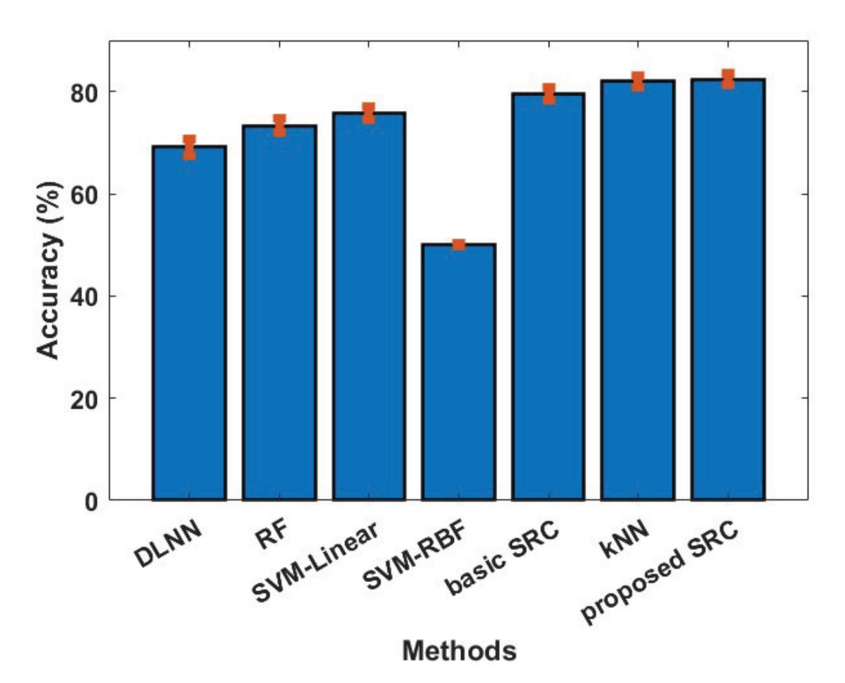
**Figure 1.** Averaged classification accuracy (with standard error) between the least and most preferred products.
In our second series of experiments (with respect to participants' preferences), we examine if the reported classifiers can discriminate between all participants' preferences (a six class classification problem), and not only between the least and most preferred 226
*Sensors* **2023**, *23*, 2480
products. In this experiment, the 10-fold cross-validation approach was used in order to examine the performance of classifiers, and this procedure has been repeated 10 times to reduce any random effects. In Figure 2, we see the average performance for each classifier. Again, we can observe that the SRC classifier provides the best performance among all the methods. The SRC achieves an average accuracy of 64.70% compared to 59.47% of basic SRC (the second best classifier). Additionally, the SVM with RBF kernel has achieved an accuracy of 43.70%, while the SVM with linear kernel has achieved accuracy of 34.54%, the kNN 53.63%, the RF 39.62%, and the DLNN 28,42%. Furthermore, we can observe here that all classifiers provide accuracy above the random level (16.67%), indicating that it is possible to distinguish between different affective states of the brain. One way ANOVA was conducted to compare the effect of the classification methods on accuracy values. The used methods were compared. There was a significant difference in the accuracy among the classification methods at the *p* < 0.05 level for the seven methods F(6,693) = 460.71, *p* < 0.001. Post hoc analysis revealed that the proposed SRC method had a significantly better accuracy than the rest of the methods. The above-reported results provide evidence supporting our hypothesis that EEG features from different brain processes lie into different linear subspaces. Finally, in Figure 2, we provide the confusion matrices for each classifier. Additionally, we calculate the class-wise recall (true positive rate), by normalizing the confusion matrix across each row, and the class-wise precision (positive predictive value), by normalizing across each column the confusion matrix. We can observe that, in the majority of classes (i.e., the participants' preferences), the proposed SRC scheme provides the best class-wise recall and the best class-wise precision. Our model achieved the highest recall and precision for the majority of classes, indicating better classification performance from the other methods.
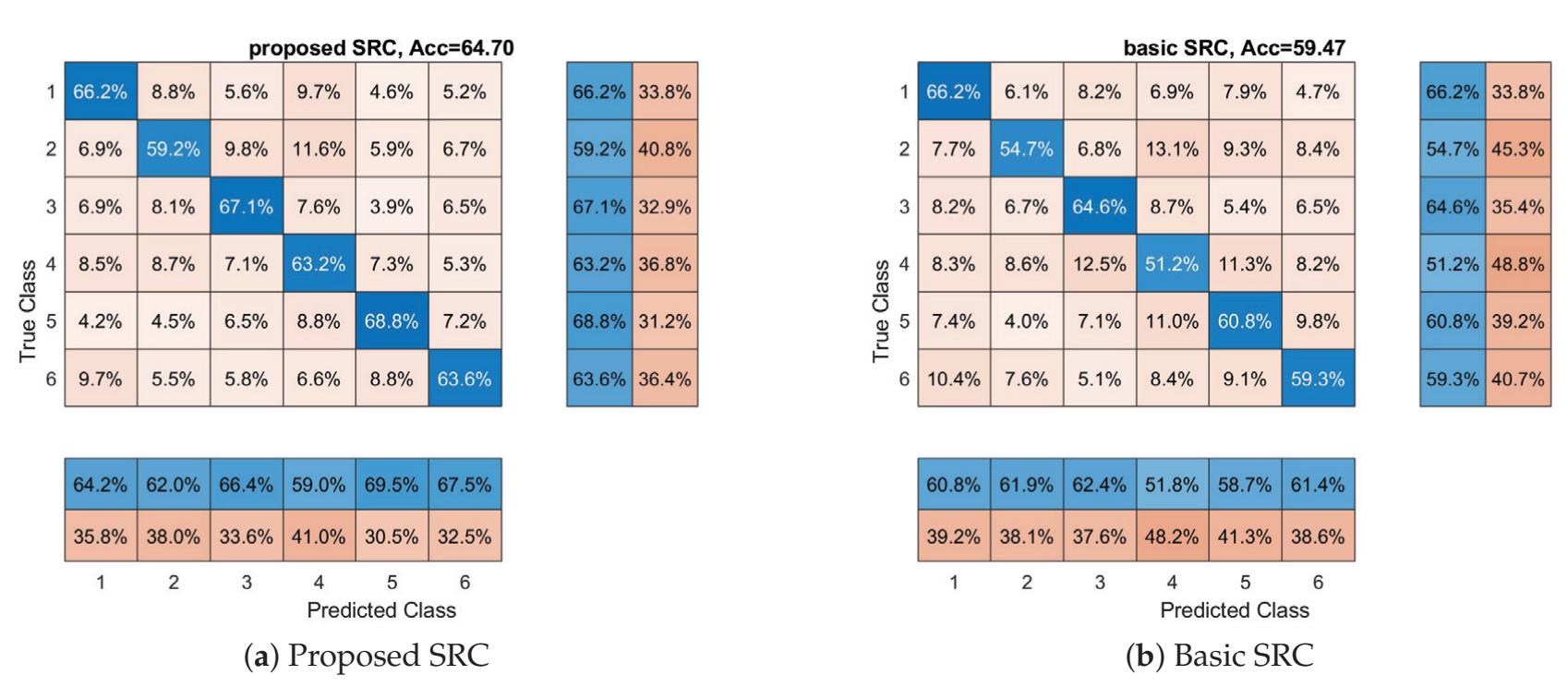
**Figure 2.** *Cont*.
227
*Sensors* **2023**, *23*, 2480
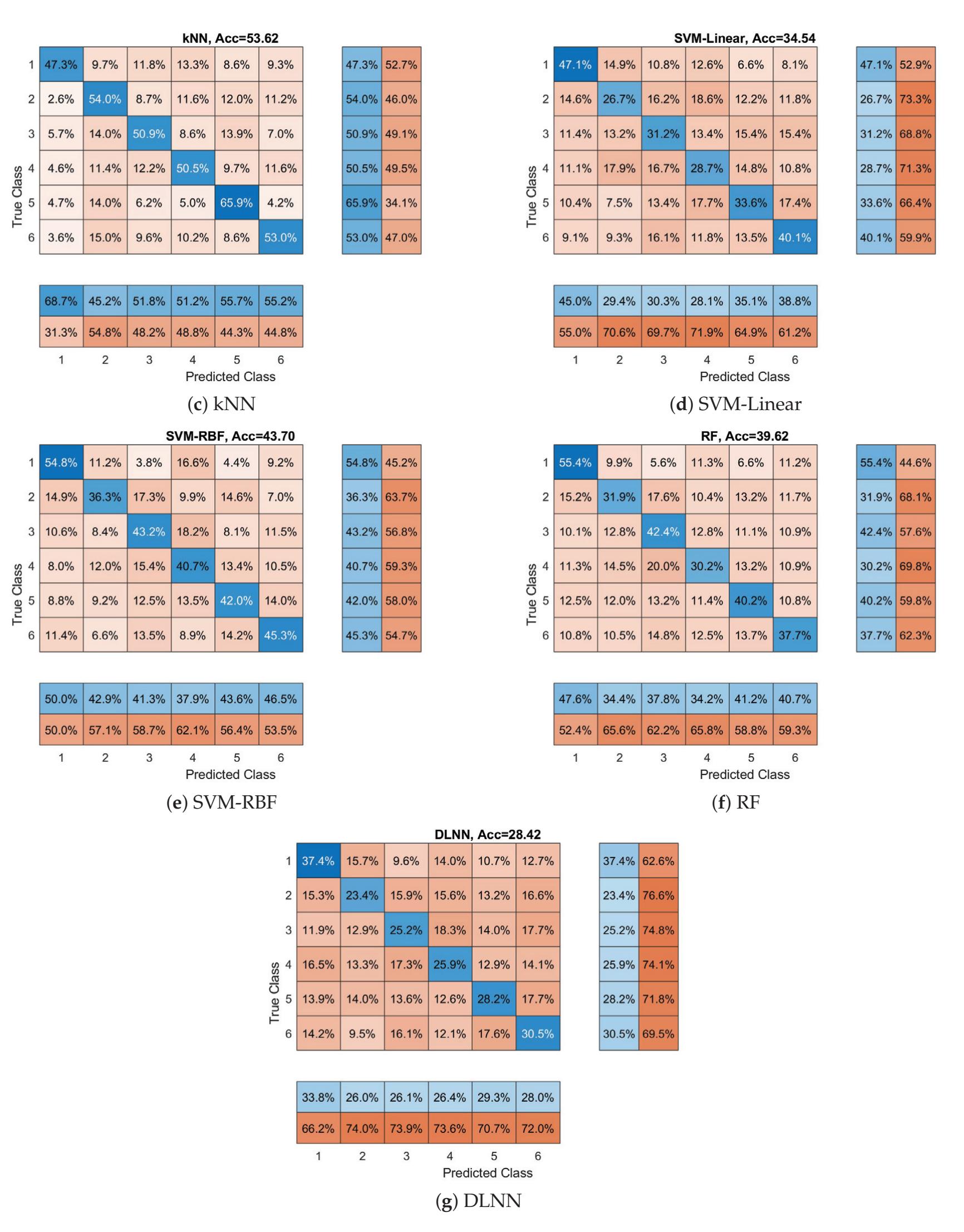
**Figure 2.** Overall accuracy and confusion matrices for each method with respect to products' preferences. Each matrix provides the overall performance of each classifier with respect to each class (in our case, product's preferences). Furthermore, class-wise precision (last two separated columns on the right) and class-wise recall (last two separated rows on the bottom) are provided.
228
*Sensors* **2023**, *23*, 2480
### 3.2. Cognitive States Recognition
Now, we will examine if classifiers can discriminate between products' ads/video (a six class classification problem) using the brain signals of the participants. The basic goal of this experiment is to examine if the cognitive states that are produced in the participant's brain when he/she watches a product's video are different among products. In this experiment, the 10-fold cross-validation approach was used and this procedure was repeated 10 times. In Figure 3, we see the average performance for each classifier. More specifically, we can observe that the proposed SRC achieves an average accuracy of 68.09% compared to 51.09%, 43.92%, 57.69%, 63.83%, 47.90%, and 37.70% of SVM-RBF, SVM-Linear, kNN, basic SRC, RF, and DLNN. Again, we can observe that the proposed SRC classifier provides the best performance among all the methods. One-way ANOVA was conducted to compare the effect of the classification methods on the accuracy values. The used methods were compared. There was a significant difference in the accuracy among the classification methods at the *p* < 0.05 level for the seven methods F(6,693) = 276.79, *p* < 0.001. The post hoc analysis revealed that the proposed SRC method had a significantly different accuracy than the rest of the methods. Furthermore, in Figure 3, we also provide the confusion matrices for each classifier with the class-wise precision and class-wise recall. The above results clearly show the superior performance of the proposed SRC scheme against the competitive methods. Again, all the classifiers provide performance above random classification (16.67%), a clear indication that, at some degree, the used marketing stimuli evoke different cognitive states in the brain of the participants. Additionally, from a neuromarketing perspective, we can observe in Figure 3 that all classifiers present their best class-wise (or *product-wise*) accuracy with respect to the first product; hence, we can conclude that the video related to this product is more easily remembered and recognized (i.e., imprinted) by the participants.
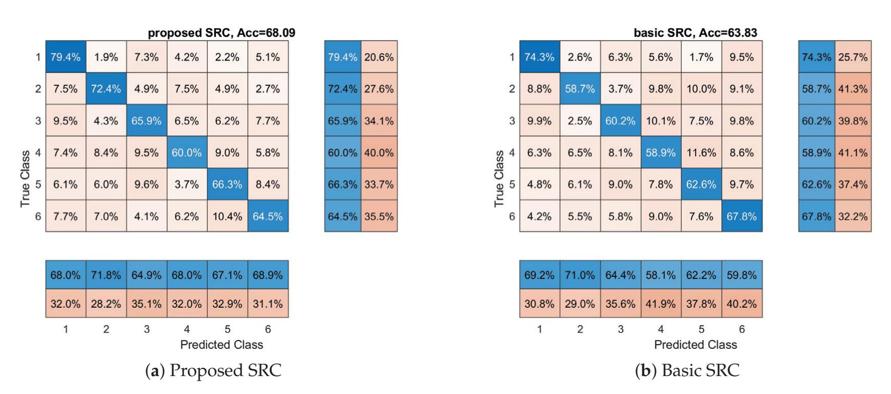
**Figure 3.** *Cont*.
229
*Sensors* **2023**, *23*, 2480
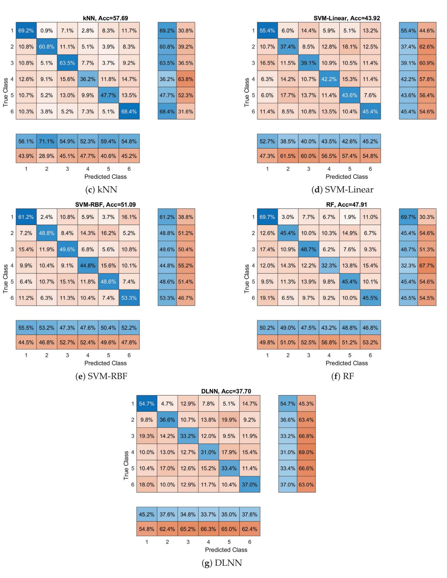
**Figure 3.** Overall accuracy and confusion matrices for each method with respect to which product the participant views. These matrices provide the performance of each classifier with respect to each class (in our case participant views). Furthermore, the class-wise precision (last two separated columns on the right) and class-wise recall (last two separated rows on the bottom) are provided.
230
*Sensors* **2023**, *23*, 2480
### 3.3. Sensitivity to the Number of Training Samples
In this subsection, we provide experimental evidence about the sensitivity of our method with respect to the number of training samples. More specifically, we perform experiments with a varying number of training samples. As a case study for these experiments, we use the binary classification problem related to the affective states recognition, and, more specifically, to the recognition of the least and most preferred products. We use the train/test split as the cross-validation approach, where we vary the size of the training set. Furthermore, we provide comparisons with the SVM-Linear, kNN, and basic SRC. These methods present the best performance among the comparative methods on our first experiment (see Figure 1). The obtained results are provided in Figure 4. We can observe that all the methods increase their performance as the size of the training set is increasing. However, we can also observe that the proposed method provides the best performance in all cases compared to other methods. It is interesting to note here that, to achieve a similar level of performance, our method needs significantly less training samples. For example, to achieve an accuracy of 75%, it needs 73 training samples, while the SVM-Linear needs 146 and the kNN around 100. Furthermore, we can observed that the basic SRC scheme is the second best method, especially for a small number of training samples, indicating that the assumption of sparse representation is valid for these kinds of data. Furthermore, comparing the proposed method with the methods presented in [13,42], we can conclude that our method needs less training samples to achieve the same level of performance. To conclude, it is obvious that the proposed method exhibits better behaviour than the other comparative methods with respect to the number of training samples.
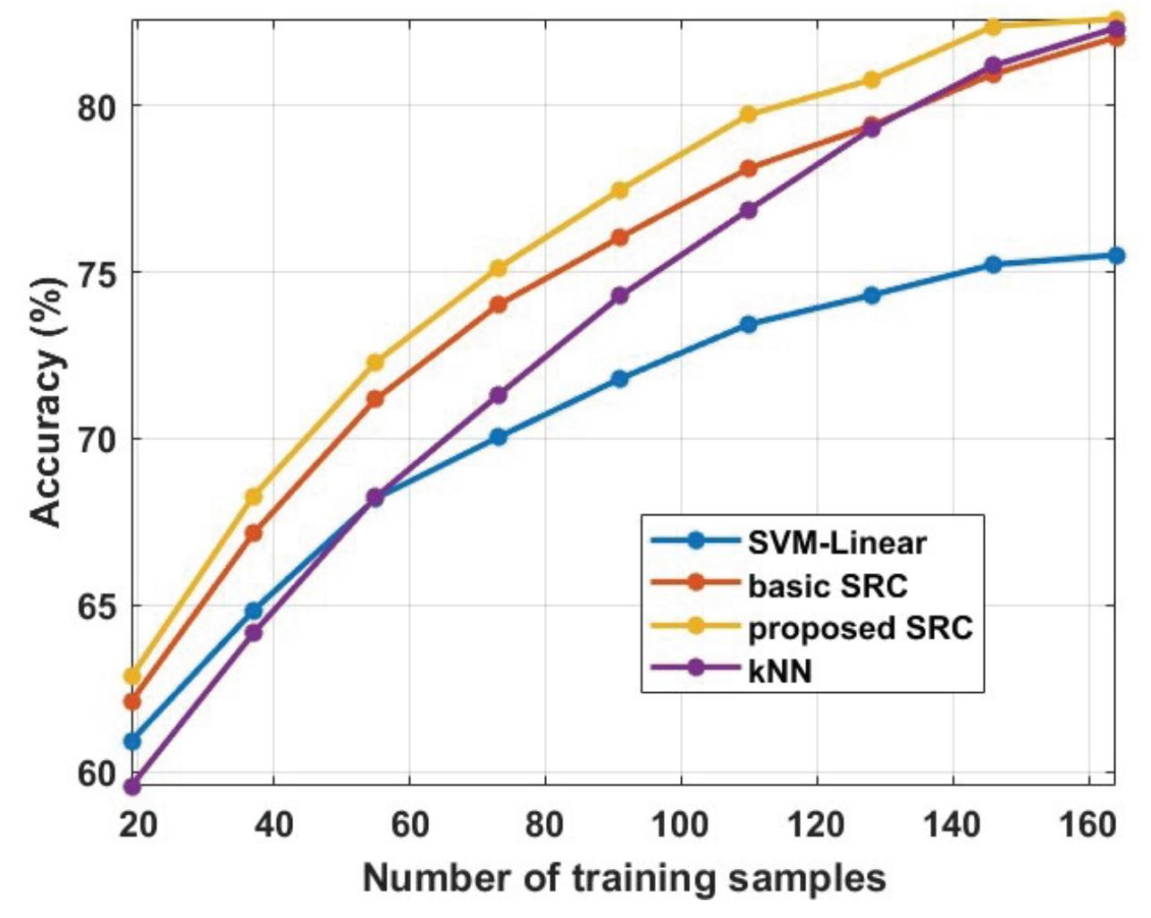
**Figure 4.** Averaged classification accuracy by changing the number of training samples from 20 to 160 training samples.
## 4. Discussion
The provided experiments have shown the superior performance of our algorithm over the SVM classifier. However, it is important to the here three basic methodological differences between the SVM classifier and the proposed SRC-based classifier. The first difference is on how the presented algorithms are using the training data. The SVM is 231
*Sensors* **2023**, *23*, 2480
an eager learner [40,41], determining the decision boundary from the training data before considering any testing sample. On the other side, the SRC classifier (similar to kNN) is a lazy learner [40,41], just storing training samples and waiting until it is given a testing sample before considering any computation, or learning. The second difference lies on how each methodology deals with what is called *linear combination*. The SVM linearly combines the features in order to provide a decision about the current testing sample. On the other side, the SRC classifier linearly combines the training samples in order to decide about the testing sample. The third difference lies on the underlying assumptions about the structure of the data. The SVM assumes that the classes are discriminated by hyperplanes, while the SRC assumes that classes lie in different subspaces; hence, a testing sample can be linearly represented more accurately by the training samples of the same class.
From the above properties, we can observe that, when a new test signal arrives, our approach needs to find the weights before deciding for the label. Instead, classifiers such as SVM just compute a linear combination since the weights are learned before processing the test signal. Hence, the computational complexity of our algorithm is considerably larger. However, we can mitigate, at some degree, for this disadvantage. More specifically, we can derive a fast version of the above algorithm adopting the fast marginal likelihood maximization procedure. This fast version provides an elegant treatment of feature vectors by adaptively constructing the dictionary matrix through three basic operators: addition, deletion, and re-estimation. More information on this subject can be found in [38,39].
One important aspect of our approach is related to the construction of the dictionary. The sparse representation modeling of data assumes an ability to describe a test sample as linear combinations of a few training samples from a training set (i.e., atoms from a pre-specified dictionary) [43]. Under this view, the choice of the training set (or dictionary) is crucial for the success of this model. In general, the choice of a proper dictionary can be performed by building a sparsifying dictionary based on a mathematical model of the data or learning a dictionary from the training set. In our work, we constructed the dictionary from the data using a simplified approach. More specifically, the dictionary was constructed by concatenating the extracted feature vectors. However, someone has the possibility to learn a specialized dictionary from the particular data using approaches such as kSVD [43]. Furthermore, features that by design lead to sparse representations could be adopted. One such case are the features based on Common Spatial Patterns (CSP). These types of features have been used under the concept of sparse representation in motor imagery problems [31]. More specifically, CSP features lead to a dictionary that partially posses the property of incoherence (i.e., incoherence between classes) [31]. A crucial property that has connections with Compressive Sensing theory. In the future, it is our intention to use the aforementioned methods for constructing a more suitable dictionary for the proposed SRC classification scheme.
In our approach, we have used features related to brain activity. These features are used to discriminate between the preferences of a participant (i.e., the least and most preferred products) and/or visual stimuli (i.e., which product's video the participant watch). However, the above features ignore, or at least they do not fully exploit, a very important property of brain that is related to the connectivity between brain's areas in response to a stimuli. Brain connectivity has shown great potential in the recognition of brain diseases [44,45] and in BCI systems [46]. Hence, future extensions of our algorithm could include features based on brain connectivity. Furthermore, an approach similar to [26] could be adopted where time–frequency (TF) maps (or features) of EEG signals are extracted and used as features. It is interesting to examine if this type of features possess similar properties to the CSP features. Furthermore, we note that we have extracted features that describe the brain activity patterns (spectral features), asymmetry between brain's areas, and correlations between the participants. We can observe that these features try to explain the different characteristics of the brain, so they can be considered as features that belong to different families. Hence, in the future, a more sophisticated fusion approach could be adopted instead of the concatenation approach.
*Sensors* **2023**, *23*, 2480
It is important to discuss some issues related to the selected channels of our work. The provided channels do not cover the entire brain; however, they are suitable for neuromarketing purposes because the electrode sites are located in the prefrontal cortex. The prefrontal cortex is associated with sustained attention, emotions, working memory, and executive planning [16,47], Furthermore, recent evidence suggests that it may be an integral part for visual perception and recognition [48]. Additionally, prefrontal EEG channels have several attractive properties for real-world applications: discreet (not clearly visible), unobtrusive, comfortable to wear, impeding the user as little as possible, and user-friendly, since they can be operated and attached by the user [49,50]. However, there is a compromise in the recording quality resulting into noisy signals, with low SNR. Clearly, more channels covering all four brain cortices could be used if someone desires to perform an intensive analysis of neural responses using the richer representations that are offered by the larger number of channels. In the current study, we demonstrate that the contribution of EEG measures to prediction with a cost-effective electrode array is possible.
Most neuromarketing-related EEG studies explore the affective states of the brain, ignoring the cognitive aspect of the problem. Identifying EEG-based discriminative features for video categorization might provide meaningful insight about the human visual perception systems [9,51]. As a consequence, it will greatly advance the performance of BCI-based applications enabling a new form of brain-based neuromarketing-related video labeling. Furthermore, during the cognitive stage of watching video commercials, the parietal region receives sensory stimuli and messages from different brain regions. During this cognitive integration, the stimulus is represented in the human brain, according to its physical characteristics or *personal experience* [22]. Additionally, in the cognitive process involved for the understanding of objects, a high-level multimodal semantic integration occurs. All the above cognitive phenomena influence the affective brain's states brought on by the video/ads and are creating an impact on the final preference decision about this video/these ads [22]. In our work, we provide evidence that the EEG signals from neuromarketing studies can be used to provide additional information to the experimenter related to the recognition of visual objects from the participant's brain. The recognition of ads using EEG data may help us to better understand the decision process inside the human brain and, potentially, it could be helpful for designing a highly robust, possibly brain-inspired model related to the human affection process with applications to neuromarketing.
## 5. Conclusions
In this work, we have proposed a new SRC-based classifier for the recognition of affective and cognitive brain states for neuromarketing purposes. More specifically, an extension of the basic SRC scheme was proposed that utilizes the graph properties of neuroimaging data. Our experiments have shown that the extended SRC classifier is capable of achieving better performance than the widely used classifiers in neuromarketing studies such as the SVM, kNN, DLNN, RF, and decoders based on Riemannian Geometry. Furthermore, based on the provided results, we can see that it is able to accurately discriminate between cognitive tasks (different products) and between affective tasks (the participants' preferences). Our experimental analysis provides evidence that EEG signals could be used for predicting consumers' preferences in neuromarketing scenarios. Our algorithm has been tested on a dataset with 33 participants, which is a suitable number for our experiments; however, a much larger number of participants is required to ensure the generalization of our work; hence, in the future, we intent to construct and release to the scientific community a new dataset related to neuromarketing and EEG. Finally, high-level future extensions of our work could include the introduction of video semantics in order to discover additional perspectives of the same dataset, and the usage of transfer learning approaches to predict the preferences of one specific participant.
233
*Sensors* **2023**, *23*, 2480
**Author Contributions:** Conceptualization, V.P.O., K.G., F.K. and S.N.; methodology, V.P.O.; software, V.P.O. and K.G.; validation, V.P.O. and F.K; data curation, V.P.O. and K.G.; formal analysis, V.P.O.; writing—original draft preparation, V.P.O.; writing—review and editing, V.P.O., K.G, F.K. and S.N.; supervision, S.N. and I.K. All authors have read and agreed to the published version of the manuscript.
**Funding:** This work was supported by the NeuroMkt project, and co-financed by the European Regional Development Fund of the EU and Greek National Funds through the Operational Program Competitiveness, Entrepreneurship and Innovation, under RESEARCH CREATE INNOVATE (T2EDK-03661).
**Institutional Review Board Statement:** Not applicable.
**Informed Consent Statement:** Not applicable.
**Data Availability Statement:** The Neuromarketing dataset can be found at https://doi.org/10.1016/ j.ijresmar.2020.10.005 (accessed on 8 January 2022).
**Conflicts of Interest:** The authors declare no conflict of interest.
## References
- 1. Lécuyer, A.; Lotte, F.; Reilly, R.; Leeb, R.; Hirose, M.; Slater, M. Brain-Computer Interfaces, Virtual Reality, and Videogames. *Computer* **2008**, *41*, 66–72. [CrossRef]
- 2. Alimardani, M.; Hiraki, K. Passive Brain-Computer Interfaces for Enhanced Human-Robot Interaction. *Front. Robot. AI* **2020**, *7*, 125. [CrossRef] [PubMed]
- 3. Gao, X.; Wang, Y.; Chen, X.; Gao, S. Interface, interaction, and intelligence in generalized brain–computer interfaces. *Trends Cogn. Sci.* **2021**, *25*, 671–684. [CrossRef]
- 4. Ramadan, R.A.; Vasilakos, A.V. Brain computer interface: Control signals review. *Neurocomputing* **2017**, *223*, 26–44. [CrossRef]
- 5. Zander, T.O.; Kothe, C. Towards passive brain–computer interfaces: Applying brain–computer interface technology to human–machine systems in general. *J. Neural Eng.* **2011**, *8*, 025005. [CrossRef] [PubMed]
- 6. Kalaganis, F.P.; Georgiadis, K.; Oikonomou, V.P.; Laskaris, N.A.; Nikolopoulos, S.; Kompatsiaris, I. Unlocking the Subconscious Consumer Bias: A Survey on the Past, Present, and Future of Hybrid EEG Schemes in Neuromarketing. *Front. Neuroergonomics* **2021**, *2*, 11. [CrossRef]
- 7. Yadava, M.; Kumar, P.; Saini, R.; Roy, P.P.; Dogra, D.P. Analysis of EEG signals and its application to neuromarketing. *Multimed. Tools Appl.* **2017**, *76*, 19087–19111. [CrossRef]
- 8. Lin, M.H.; Cross, S.; Jones, W.; Childers, T. Applying EEG in consumer neuroscience. *Eur. J. Mark.* **2018**, *52*, 66–91. [CrossRef]
- 9. Jiang, J.; Fares, A.; Zhong, S.H. A Context-Supported Deep Learning Framework for Multimodal Brain Imaging Classification. *IEEE Trans. -Hum.-Mach. Syst.* **2019**, *49*, 611–622. [CrossRef]
- 10. Hakim, A.; Levy, D. A gateway to consumers' minds: Achievements, caveats, and prospects of electroencephalography-based prediction in neuromarketing. *WIREs Cogn. Sci.* **2019**, *10*, e1485. [CrossRef]
- 11. Braeutigam, S.; Rose, S.; Swithenby, S.; Ambler, T. The distributed neuronal systems supporting choice-making in real-life situations: differences between men and women when choosing groceries detected using magnetoencephalography. *Eur. J. Neurosci.* **2004**, *20*, 293–302. [CrossRef] [PubMed]
- 12. Khushaba, R.N.; Wise, C.; Kodagoda, S.; Louviere, J.; Kahn, B.E.; Townsend, C. Consumer neuroscience: Assessing the brain response to marketing stimuli using electroencephalogram (EEG) and eye tracking. *Expert Syst. Appl.* **2013**, *40*, 3803–3812. [CrossRef]
- 13. Hakim, A.; Klorfeld, S.; Sela, T.; Friedman, D.; Shabat-Simon, M.; Levy, D.J. Machines learn neuromarketing: Improving preference prediction from self-reports using multiple EEG measures and machine learning. *Int. J. Res. Mark.* **2021**, *38*, 770–791. . [CrossRef]
- 14. Shah, S.M.A.; Usman, S.M.; Khalid, S.; Rehman, I.U.; Anwar, A.; Hussain, S.; Ullah, S.S.; Elmannai, H.; Algarni, A.D.; Manzoor, W. An Ensemble Model for Consumer Emotion Prediction Using EEG Signals for Neuromarketing Applications. *Sensors* **2022**, *22*, 9744. [CrossRef]
- 15. Wei, Z.; Wu, C.; Wang, X.; Supratak, A.; Wang, P.; Guo, Y. Using Support Vector Machine on EEG for Advertisement Impact Assessment. *Front. Neurosci.* **2018**, *12*, 76. [CrossRef]
- 16. Palmiero, M.; Piccardi, L. Frontal EEG asymmetry of mood: A mini-review. *Front. Behav. Neurosci.* **2017**, *11*, 8. [CrossRef]
- 17. Ravaja, N.; Somervuori, O.; Salminen, M. Predicting Purchase Decision: The Role of Hemispheric Asymmetry over the Frontal Cortex. *J. Neurosci. Psychol. Econ.* **2013**, *6*, 1. [CrossRef]
- 18. Ohme, R.; Reykowska, D.; Wiener, D.; Choromanska, A. Application of frontal EEG asymmetry to advertising research. *J. Econ. Psychol.* **2010**, *31*, 785–793. [CrossRef]
- 19. Shestyuk, A.Y.; Kasinathan, K.; Karapoondinott, V.; Knight, R.; Gurumoorthy, R. Individual EEG measures of attention, memory, and motivation predict population level TV viewership and Twitter engagement. *PLoS ONE* **2019**, *14*, e0214507. [CrossRef]
234
*Sensors* **2023**, *23*, 2480
- 20. Vecchiato, G.; Toppi, J.; Astolfi, L.; Fallani, F.D.V.; Cincotti, F.; Mattia, D.; Bez, F.; Babiloni, F. Spectral EEG frontal asymmetries correlate with the experienced pleasantness of TV commercial advertisements. *Med. Biol. Eng. Comput.* **2011**, *49*, 579–583. [CrossRef]
- 21. Barnett, S.; Cerf, M. A Ticket for Your Thoughts: Method for Predicting Content Recall and Sales Using Neural Similarity of Moviegoers. *J. Consum. Res.* **2017**, *44*, 160–181. [CrossRef]
- 22. Wang, R.W.; Chang, Y.C.; Chuang, S.W. EEG Spectral Dynamics of Video Commercials: Impact of the Narrative on the Branding Product Preference. *Sci. Rep.* **2016**, *6*, 36487. [CrossRef] [PubMed]
- 23. Vecchiato, G.; Astolfi, L.; Vico, F.D.; Cincotti, F.; Mattia, D.; Salinari, S.; Soranzo, R.; Babiloni, F. Changes in Brain Activity During the Observation of TV Commercials by Using EEG, GSR and HR Measurements. *Brain Topogr.* **2010**, *23*, 165–179. [CrossRef] [PubMed]
- 24. Huang, J.; Xu, X.; Zhang, T. Emotion classification using deep neural networks and emotional patches. In Proceedings of the 2017 IEEE International Conference on Bioinformatics and Biomedicine (BIBM), Kansas City, MO, USA, 13–16 November 2017; pp. 958–962. [CrossRef]
- 25. Xu, H.; Plataniotis, K.N. Affective states classification using EEG and semi-supervised deep learning approaches. In Proceedings of the 2016 IEEE 18th International Workshop on Multimedia Signal Processing (MMSP), Montreal, QC, Canada, 21–23 September 2016; pp. 1–6. [CrossRef]
- 26. Ieracitano, C.; Morabito, F.C.; Hussain, A.; Mammone, N. A Hybrid-Domain Deep Learning-Based BCI for Discriminating Hand Motion Planning from EEG Sources. *Int. J. Neural Syst.* **2021**, *31*, 2150038. [CrossRef] [PubMed]
- 27. Gong, S.; Xing, K.; Cichocki, A.A.; Li, J. Deep Learning in EEG: Advance of the Last Ten-Year Critical Period. *IEEE Trans. Cogn. Dev. Syst.* **2022**, *14*, 348–365. [CrossRef]
- 28. Hamilton, W.L.; Ying, R.; Leskovec, J. Representation Learning on Graphs: Methods and Applications. *arXiv* **2017**, arXiv:1709.05584.
- 29. Wright, J.; Yang, A.Y.; Ganesh, A.; Sastry, S.S.; Ma, Y. Robust Face Recognition via Sparse Representation. *IEEE Trans. Pattern Anal. Mach. Intell.* **2009**, *31*, 210–227. [CrossRef]
- 30. Shen, C.; Chen, L.; Dong, Y.; Priebe, C. Sparse Representation Classification Beyond *l*1 Minimization and the Subspace Assumption. *IEEE Trans. Inf. Theory* **2020**, *66*, 5061–5071. [CrossRef]
- 31. Oikonomou, V.P.; Nikolopoulos, S.; Kompatsiaris, I. Robust Motor Imagery Classification Using Sparse Representations and Grouping Structures. *IEEE Access* **2020**, *8*, 98572–98583. [CrossRef]
- 32. Shu, T.; Zhang, B.; Tang, Y. Sparse Supervised Representation-Based Classifier for Uncontrolled and Imbalanced Classification. *IEEE Trans. Neural Netw. Learn. Syst.* **2020**, *31*, 2847–2856. [CrossRef]
- 33. Shin, Y.; Lee, S.; Lee, J.; Lee, H.N. Sparse representation-based classification scheme for motor imagery-based brain–computer interface systems. *J. Neural Eng.* **2012**, *9*, 056002. [CrossRef] [PubMed]
- 34. Oikonomou, V.P.; Nikolopoulos, S.; Kompatsiaris, I. Sparse Graph-based Representations of SSVEP Responses Under the Variational Bayesian Framework. In Proceedings of the 2021 IEEE 21st International Conference on Bioinformatics and Bioengineering (BIBE), Kragujevac, Serbia, 25–27 October 2021; pp. 1–6. [CrossRef]
- 35. Badre, D.; Nee, D.E. Frontal Cortex and the Hierarchical Control of Behavior. *Trends Cogn. Sci.* **2018**, *22*, 170–188. [CrossRef]
- 36. Davenport, M.A.; Duarte, M.F.; Eldar, Y.C.; Kutyniok, G. Introduction to compressed sensing. In *Compressed Sensing: Theory and Applications*; Eldar, Y.C., Kutyniok, G., Eds.; Cambridge University Press: Cambridge, UK, 2012; pp. 1–64. [CrossRef]
- 37. Oikonomou, V.P.; Nikolopoulos, S.; Kompatsiaris, I. A Novel Compressive Sensing Scheme under the Variational Bayesian Framework. In Proceedings of the 27th European Signal Processing Conference (EUSIPCO 2019), Corunna, Spain, 2–6 September 2019; pp. 1–4.
- 38. Tipping, M.E. Sparse Bayesian Learning and the Relevance Vector Machine. *J. Mach. Learn. Res.* **2001**, *1*, 211–244.
- 39. Jiang, B.; Chen, H.; Yuan, B.; Yao, X. Scalable Graph-Based Semi-Supervised Learning through Sparse Bayesian Model. *IEEE Trans. Knowl. Data Eng.* **2017**, *29*, 2758–2771. [CrossRef]
- 40. Alpaydin, E. *Introduction to Machine Learning*, 3rd ed.; The MIT Press: Cambridge, UK, 2014.
- 41. Murphy, K.P. *Machine Learning: A Probabilistic Perspective*; MIT Press: Cambridge, UK, 2022.
- 42. Georgiadis, K.; Kalaganis, F.P.; Oikonomou, V.P.; Nikolopoulos, S.; Laskaris, N.A.; Kompatsiaris, I. RNeuMark: A Riemannian EEG Analysis Framework for Neuromarketing. *Brain Inform.* **2022**, *9*, 22. [CrossRef] [PubMed]
- 43. Rubinstein, R.; Bruckstein, A.M.; Elad, M. Dictionaries for Sparse Representation Modeling. *Proc. IEEE* **2010**, *98*, 1045–1057. [CrossRef]
- 44. Fornito, A.; Bullmore, E.T. Connectomics: A new paradigm for understanding brain disease. *Eur. Neuropsychopharmacol.* **2015**, *25*, 733–748. [CrossRef]
- 45. Lazarou, I.; Georgiadis, K.; Nikolopoulos, S.; Oikonomou, V.P.; Tsolaki, A.; Kompatsiaris, I.; Tsolaki, M.; Kugiumtzis, D. A Novel Connectome-based Electrophysiological Study of Subjective Cognitive Decline Related to Alzheimer's Disease by Using Resting-state High-density EEG EGI GES 300. *Brain Sci.* **2020**, *10*, 392. [CrossRef] [PubMed]
- 46. Hamedi, M.; Salleh, S.H.; Noor, A.M. Electroencephalographic Motor Imagery Brain Connectivity Analysis for BCI: A Review. *Neural Comput.* **2016**, *28*, 999–1041. [CrossRef]
- 47. Fuster, J.M. The Prefrontal Cortex Makes the Brain a Preadaptive System. *Proc. IEEE* **2014**, *102*, 417–426. [CrossRef]
235
*Sensors* **2023**, *23*, 2480
- 48. Romanski, L.M.; Chafee, M.V. A View from the Top: Prefrontal Control of Object Recognition. *Neuron* **2021**, *109*, 6–8. [CrossRef] [PubMed]
- 49. Kidmose, P.; Looney, D.; Ungstrup, M.; Rank, M.L.; Mandic, D.P. A Study of Evoked Potentials From Ear-EEG. *IEEE Trans. Biomed. Eng.* **2013**, *60*, 2824–2830. [CrossRef] [PubMed]
- 50. Oikonomou, V.P. An Adaptive Task-Related Component Analysis Method for SSVEP Recognition. *Sensors* **2022**, *22*, 7715. [CrossRef] [PubMed]
- 51. Spampinato, C.; Palazzo, S.; Kavasidis, I.; Giordano, D.; Souly, N.; Shah, M. Deep Learning Human Mind for Automated Visual Classification. In Proceedings of the 2017 IEEE Conference on Computer Vision and Pattern Recognition (CVPR), Honolulu, HI, USA, 21–26 July 2017; pp. 4503–4511. [CrossRef]
**Disclaimer/Publisher's Note:** The statements, opinions and data contained in all publications are solely those of the individual author(s) and contributor(s) and not of MDPI and/or the editor(s). MDPI and/or the editor(s) disclaim responsibility for any injury to people or property resulting from any ideas, methods, instructions or products referred to in the content.
236


*Article*
# Extraction of Individual EEG Gamma Frequencies from the Responses to Click-Based Chirp-Modulated Sounds
**Aurimas Mockeviˇcius 1, Yusuke Yokota 2, Povilas Tarailis 1, Hatsunori Hasegawa 2, Yasushi Naruse 2 and Inga Griškova-Bulanova 1,\***
- 1 Institute of Biosciences, Life Sciences Centre, Vilnius University, Sauletekio av. 7, LT-10257 Vilnius, Lithuania ˙
- 2 Center for Information and Neural Networks (CiNet), National Institute of Information and Communications Technology, Saka University, Kobe 651-2492, Hyogo, Japan
- **\*** Correspondence: i.griskova@gmail.com or inga.griskova-bulanova@gf.vu.lt; Tel.: +370-6-711-0954
**Abstract:** Activity in the gamma range is related to many sensory and cognitive processes that are impaired in neuropsychiatric conditions. Therefore, individualized measures of gamma-band activity are considered to be potential markers that reflect the state of networks within the brain. Relatively little has been studied in respect of the individual gamma frequency (IGF) parameter. The methodology for determining the IGF is not well established. In the present work, we tested the extraction of IGFs from electroencephalogram (EEG) data in two datasets where subjects received auditory stimulation consisting of clicks with varying inter-click periods, covering a 30–60 Hz range: in 80 young subjects EEG was recorded with 64 gel-based electrodes; in 33 young subjects, EEG was recorded using three active dry electrodes. IGFs were extracted from either fifteen or three electrodes in frontocentral regions by estimating the individual-specific frequency that most consistently exhibited high phase locking during the stimulation. The method showed overall high reliability of extracted IGFs for all extraction approaches; however, averaging over channels resulted in somewhat higher reliability scores. This work demonstrates that the estimation of individual gamma frequency is possible using a limited number of both the gel and dry electrodes from responses to click-based chirp-modulated sounds.
**Keywords:** individual gamma frequency (IGF); auditory steady-state response (ASSR); dry electrodes
#### **Citation:** Mockeviˇcius, A.; Yokota, Y.; Tarailis, P.; Hasegawa, H.; Naruse, Y.; Griškova-Bulanova, I. Extraction of Individual EEG Gamma Frequencies from the Responses to Click-Based Chirp-Modulated Sounds. *Sensors* **2023**, *23*, 2826. https://doi.org/ 10.3390/s23052826
Academic Editors: Yifan Zhao, Yuzhu Guo and Fei He
Received: 31 December 2022 Revised: 2 March 2023 Accepted: 2 March 2023 Published: 4 March 2023

**Copyright:** © 2023 by the authors. Licensee MDPI, Basel, Switzerland. This article is an open access article distributed under the terms and conditions of the Creative Commons Attribution (CC BY) license (https:// creativecommons.org/licenses/by/ 4.0/).
## 1. Introduction
A great interest in individualized markers of brain activity that have potential clinical or neuro-technological applications has recently emerged. This attention has largely been drawn to electroencephalography (EEG), which provides cheap and fast assessment opportunities which are applicable even outside the laboratory in ecologically valid settings. The analysis of the signal offers large possibilities with a focus on versatile domains and functional outcomes. Several authors have addressed individual resonant frequencies, i.e., the largest frequencies of the activity of subjects, as a reflection of the state of neural networks relating them to certain functional manifestations. To illustrate, peak alpha frequencies have been shown to be related to performance in cognitive tasks [1,2], whereas peak theta frequencies were proposed to relate to cognitive control [3]. Similarly, peak frequencies in the gamma range were addressed. The gamma-range activity has been argued to be important for many cognitive and sensory processes and is frequently impaired in neuropsychiatric conditions. For example, the preferred frequencies in the gamma range were related to the ability to detect a gap in the sounds, i.e., to the temporal sampling rate in the auditory system [4,5]. Additionally, peak frequencies in the gamma range were shown to decline with age [6,7] and to "slow down" in subjects with developmental dyslexia [8], patients with schizophrenia [9,10], or Alzheimer's disease [6]. This suggests that peak gamma frequencies might have a physiological meaning and deserve further investigation.
*Sensors* **2023**, *23*, 2826. https://doi.org/10.3390/s23052826 https://www.mdpi.com/journal/sensors
237
*Sensors* **2023**, *23*, 2826
However, since a prominent peak in the gamma activity is usually not observed in the EEG frequency spectra, determining individual-specific dominant gamma frequency (individual gamma frequency, IGF) is not a straightforward task. It is not entirely clear what is the best method of measurement for gamma range preferred frequencies. Attempts were made to extract it from resting-state EEG data [6], from a response to transient sensory stimuli [11,12], or in response to some meaningful cognitive tasks and related events [13,14]. Alternatively, the periodic stimulation testing of the most preferred frequency, defined as generating the largest response, was employed utilizing an auditory steady-state approach. To illustrate, Zaehle et al. stimulated using amplitude-modulate sounds at single frequencies spanning a 20–100 Hz range and estimated the preferred gamma frequencies to be around 30–60 Hz with a peak at 48 Hz [15]. Similarly, Gransier et al. tested a range of between 0.5 and 100 Hz showing that peak was within the 30–60 Hz range, with a mean of 45 Hz [16]. However, stimulation with single frequencies is time-consuming and problematic for clinical assessment; thus more elaborate approaches need to be developed. As an alternative, a chirp-based stimulation was proposed, demonstrating its capability to detect peak responses in the gamma range [17,18]. Chirp sounds represent a stimulation type where the amplitude modulation of the carrier covers certain frequency ranges of interest. However, amplitude-modulated sounds are known to evoke less pronounced EEG responses [19]. To utilize the benefits of the click-based stimulation that produces strong brain responses, we recently tested the ability of stimuli composed of single clicks when spaced in a logarithmic manner to evoke gamma-range responses [20]. This approach demonstrated that in response to stimulation, a peak in the gamma range could be observed, and responses at the peak were related to certain cognitive abilities, namely, the time needed to perform complex information-processing tasks [20,21].
The abovementioned works were performed in laboratory settings using researchgrade EEG equipment. Nevertheless, modern experimental situations require that the methods work in less controlled experimental settings, e.g., on the data of a small number of dry EEG channels that allow for fast assessment. This would enable easier translational application and assessment in more naturalistic settings.
In this work, we tested whether it was possible to reliably extract individual gamma peak information from the responses to auditory chirp-based stimulations collected with research-grade EEG equipment and dense electrode placement over the region of interest where a response was observed. Then, we tested the approach on data collected with custom-made dry EEG electrodes and a low number of EEG channels. We focused on the estimation of IGF based on the phase-locking measure that was shown to produce the strongest and most reliable results for classical auditory-steady state responses [22] and more pronounced results for click-based chirp stimulation [20,21].
## 2. Materials and Methods
### 2.1. Participants
A group of 80 young participants (42 females, 2 left-handed; mean age ± SD: 26.07 ± 4.28) without a reported history of psychiatric and neurological disorders participated in the study using a high-density EEG system. The hearing thresholds of all the subjects were within the normal range (<25 dB HL at octave frequencies). Participants abstained from alcohol 24 h prior to the testing and did not consume nicotine and caffeine-containing drinks for at least one hour prior to the experiment. The study was approved by the Vilnius Regional Biomedical Research Ethics Committee (no. 2020/3-1213-701), and all participants provided their written informed consent.
A group of 33 young subjects (15 females; mean age ± SD: 27.8 ± 5.85) without a reported history of psychiatric and neurological disorders participated in this study utilizing a custom-made dry electrode EEG system. All subjects had normal hearing along with normal or corrected-to-normal vision. Subjects provided written informed consent after the procedural details had been explained and before the experiment. All experimental procedures were approved by the Ethics Committee for Human and Animal Research of 238
*Sensors* **2023**, *23*, 2826
the National Institute of Information and Communications Technology (no. B210152204). The experiment was performed in accordance with the ethical standards described in the Declaration of Helsinki.
### 2.2. EEG Acquisition
A 64-channel EEG signal was recorded with an ANT device (ANT Neuro, Hengelo, The Netherlands) and WaveGuard EEG gel-based cap with integrated Ag/AgCl electrodes which were placed according to the 10-10 International electrode placement system. Mastoids were used as a reference; the ground electrode was attached close to Fz. Impedance was kept below 20 kΩ, and the sampling rate was set at 1024 Hz. Simultaneously, vertical and horizontal electro-occulograms (VEOG and HEOG) were recorded from above and below the left eye and from the right and left outer canthi.
The 3-channel EEG data were collected using a wireless portable system (PolymateMini AP108, Miyuki Giken Co., Ltd., Tokyo, Japan) with three active dry electrodes (Unique Medical Co., Ltd., Tokyo, Japan) [23] positioned at FC3, FCz, and FC4 according to the 10–20 International electrode placement system. The right mastoid was used as a reference; the ground electrode was attached to the left mastoid. The sampling rate was set at 500 Hz. Simultaneously, vertical and horizontal electro-occulograms (VEOG and HEOG) were recorded from above and at the side of the left eye.
### 2.3. Auditory Stimulation
Stimulus trains were created of single identical 1.5 ms white-noise bursts of alternating polarity spaced with changing inter-click periods to cover a range from 30 to 60 Hz in a decreasing-then-increasing order. The duration of the stimulus train was 1500 ms, and 200 repetitions were presented with 700–1000 ms inter-stimulus intervals. The schematic representation of the sounds used is presented in Figure 1A. The auditory stimuli were designed in the Matlab 2014 environment (The MathWorks, Inc., Natick, MA, USA) and presented binaurally through Shure SE215 earphones (in the 64-channel group) and through RHA MA750 earphones (in three dry electrode groups). The sound pressure level was set at 60 dB.
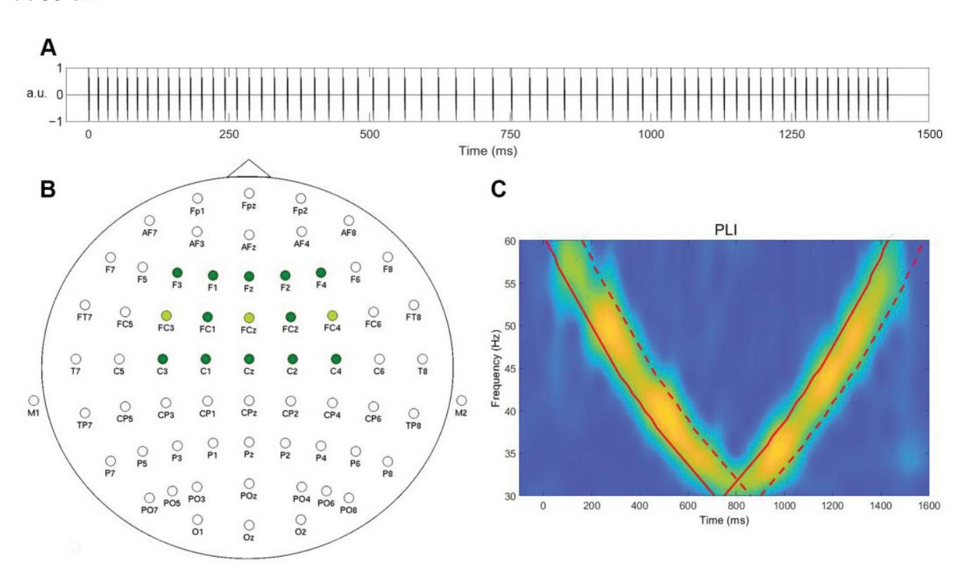
**Figure 1.** (**A**) A schematic representation of the sound stimulus used in this study. (**B**) Electrode placement for 64- and 3-channel systems. Channels used for analysis are colored in green. (**C**) A schematic representation of time-window definition for the calculation of IGFs from PLI. The bold red line indicates the timing of the stimulation; the red dashed line denotes the edge of averaging window (+150 ms). a.u.—arbitrary units.
239
*Sensors* **2023**, *23*, 2826
### 2.4. EEG Processing
The 64-channel EEG data were pre-processed in EEGLAB for MatLab© [24] in a manner as described in previous research [20]. The power-line noise was removed using multi-tapering and Thomas F-statistics (CleanLine plugin for EEGLAB). The data were visually inspected, and channels with substantial noise (shift, movements) were removed. Further, EEG data were submitted to an independent component analysis (ICA) that was performed with the ICA-implementation of EEGLAB ('runica' with default settings [25,26]) after Independent components relating to eye movements (blinks and saccades), and ECG were removed. The removed channels were then reconstructed using a 3D spherical spline method [27].
The 3-channel EEG data were offline pre-processed in EEGLAB for MatLab© [24]. An ICA was performed with the ICA implementation of EEGLAB ('runica' with default settings) after the visual inspection. Independent components related to eye movements (blinks and saccades) were removed.
### 2.5. Individual Gamma Frequency Extraction
The analysis of all the data was run using Fieldtrip [28] functions in MATLAB R2020a. Time-frequency transformation using a complex Morlet wavelet (14 cycles) was applied to the signal within a 1–120 Hz range. The phase-locking index (PLI) was used as a measure of interest and was known to be least sensitive to noise and produced the most stable results. To create responses for each subject, 100 iterations were run with 100 randomly selected epochs. In the 64-channel group, electrodes covering the frontocentral region where a gamma response to auditory stimulations was consistently observed and selected for the analysis (Figure 1B). For the 3-channel data, all electrodes were included in the analysis. The responses were averaged within 150 ms time intervals for each frequency from 30 to 60 Hz, in steps of 1 Hz. The averaging windows (marked with a red dashed line in Figure 1C) were selected based on the time onset of the corresponding frequency in the chirp-like stimulus (red bold line in Figure 1C), both in the chirp-down and chirp-up periods (Figure 1C).
Several IGF estimation approaches were tested. First, different sets of channels were selected for 64-channel data: 15 channels (F3, F1, Fz, F2, F4, FC3, FC1, FCz, FC2, FC4, C3, C1, Cz, C2, and C4) or 3 channels (FC3, FCz, and FC4). Secondly, for both sets of selected channels, the PLI values in chirp-down and chirp-up periods were either averaged together to obtain a single IGF estimate for each frequency or were analyzed separately to obtain two IGF estimates–one for the down part and one for the up part. This was conducted in order to account for the possibility that "slowing" or "speeding" (frequency change) could depend on the direction of stimulation. These 6 approaches are further referred to as "IGF extraction condition": electrodes kept, down-up; electrodes averaged, down-up; electrodes kept, down; electrodes kept, up; electrodes averaged, down; electrodes averaged, up. Furthermore, the outputs within each selected channel were also averaged or kept separated. In all of these approaches, 5 dominant frequencies within a 30–60 Hz range with the highest PLI values were extracted for each trial iteration (and channel, if channels were not averaged), resulting in a trial iteration (×channel) × the top 5 frequencies of the matrix for each subject.
To estimate the most prevalent IGFs, the mode was computed from all the values within the matrix for each subject following the reasoning of Bjeki´c et al. [29]. The participant-level reliability of IGF was calculated as the ratio between the number of IGF values within the whole matrix and the total number of cells within the matrix after excluding the last dimension, which represented the top 5 frequencies. The rationale behind choosing this divisor was that any frequency value could be present only once among a single set of the top 5 frequencies, thus excluding the last dimension, which allowed one to estimate how consistently the IGF value appeared among the dominant 5 frequencies in each trial iteration and (if not averaged) each channel. The computed IGF reliability ratios of all subjects were further divided into ranges: singular IGF (>0.8), high IGF reliability 240
*Sensors* **2023**, *23*, 2826
(0.51–0.8), medium IGF reliability (0.31–0.5), low IGF reliability (0.16–0.3), and no IGF (≤0.15). The example of IGF estimation from a single subject is presented in Figure 2. To further compare the reliability ratios across different IGF extraction conditions, a nonparametric Friedman test and post hoc Wilcoxon pairwise comparisons with Bonferroni correction were applied.
| Subject 1 (F, 25) | | | | | |
|-------------------|-----------------------------------------|-----|-----|-----|-----|
| Trial iterations | 5 frequencies (Hz) with the highest PLI | | | | |
| | 1 | 2 | 3 | 4 | 5 |
| 1 | 39 | 40 | 38 | 41 | 37 |
| 2 | 41 | 40 | 42 | 39 | 43 |
| 3 | 42 | 41 | 43 | 40 | 39 |
| 4 | 39 | 38 | 40 | 41 | 37 |
| 5 | 40 | 39 | 41 | 38 | 42 |
| 6 | 41 | 40 | 42 | 39 | 43 |
| 7 | 42 | 41 | 43 | 40 | 39 |
| 8 | 42 | 41 | 40 | 39 | 43 |
| 9 | 39 | 40 | 41 | 38 | 42 |
| 10 | 42 | 41 | 39 | 38 | 43 |
| ... | ... | ... | ... | ... | ... |
| 100 | 40 | 41 | 39 | 38 | 42 |
| Subject 2 (M, 22) | | | | | |
|-----------------------------------------|-----|-----|-----|-----|-----|
| 5 frequencies (Hz) with the highest PLI | | | | | |
| Trial iterations | 1 | 2 | 3 | 4 | 5 |
| 1 | 36 | 37 | 35 | 38 | 39 |
| 2 | 36 | 37 | 32 | 35 | 33 |
| 3 | 32 | 31 | 33 | 36 | 37 |
| 4 | 36 | 37 | 35 | 33 | 38 |
| 5 | 36 | 37 | 35 | 38 | 34 |
| 6 | 37 | 36 | 38 | 39 | 35 |
| 7 | 37 | 38 | 36 | 39 | 35 |
| 8 | 36 | 37 | 35 | 38 | 39 |
| 9 | 37 | 36 | 38 | 35 | 39 |
| 10 | 32 | 36 | 37 | 33 | 35 |
| ... | ... | ... | ... | ... | ... |
| 100 | 35 | 36 | 33 | 32 | 34 |
**Figure 2.** An example of IGF estimation on an average of 15 channels and averaged chirp-down and chirp-up parts in two subjects: the matrix of 100 trial iterations and 5 frequencies displaying the highest PLI response. The extracted IGF is marked in red.
## 3. Results
For visualization purposes, the time-frequency plots of PLIs for two representative subjects of data averaged over 15 gel electrodes with corresponding topographies at estimated IGF for chirp-down, chirp-up, and both parts averaged (A), and time-frequency plots of PLIs for two representative subjects for data averaged over 3 dry electrodes (B) are presented in Figure 3.
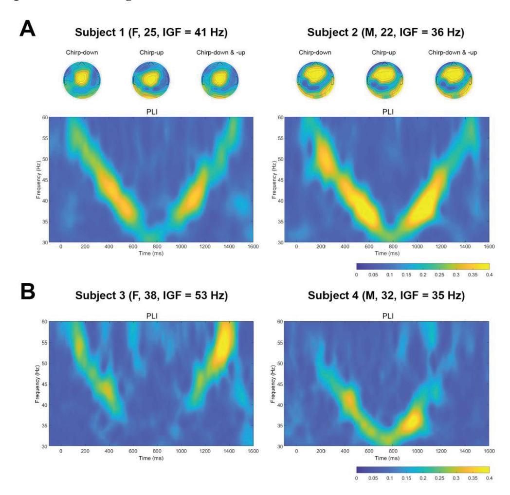
**Figure 3.** Example of time-frequency plots of PLIs. (**A**) Time-frequency plots of PLIs for two subjects from 15 gel electrodes data. Topoplots at IGF were created separately for chirp-down, chirp-up, and the averaging of both parts. (**B**) Time-frequency plots of PLIs for two subjects from three dry electrodes data.
241
*Sensors* **2023**, *23*, 2826
### 3.1. 64-channel Gel Electrode System
The descriptive statistics of IGF estimation for all the tested conditions are presented in Table 1. Alongside the mean values, ranges of estimated IGF values and reliability scores for every method tested are presented.
**Table 1.** Descriptive statistics of the IGF estimations and IGF reliability intervals from 64-channel gel electrode data.
| | IGF Extraction Condition | Descriptive Statistics | | | | Reliability Intervals * | | | | |
|-------------|------------------------------|------------------------|----------------------|---------------------|----------------------|-------------------------|-------------|---------------|------------|---------------|
| | | Mean
IGF (Hz) | IGF
Range
(Hz) | Mean
Reliability | Reliability
Range | Singular
IGF (n) | High
(n) | Medium
(n) | Low
(n) | No IGF
(n) |
| 15 channels | Electrodes kept, down-up | 37 (±4) | 30–47 | 0.67 (±0.16) | 0.27–0.98 | 15 | 47 | 17 | 1 | 0 |
| | Electrodes averaged, down-up | 37 (±4) | 30–47 | 0.89 (±0.12) | 0.47–1.0 | 62 | 17 | 1 | 0 | 0 |
| | Electrodes kept, down | 37 (±5) | 31–53 | 0.59 (±0.16) | 0.29–0.95 | 11 | 42 | 26 | 1 | 0 |
| | Electrodes kept, up | 37 (±3) | 30–45 | 0.66 (±0.13) | 0.32–0.97 | 10 | 59 | 11 | 0 | 0 |
| | Electrodes averaged, down | 38 (±5) | 31–52 | 0.83 (±0.15) | 0.51–1.0 | 47 | 33 | 0 | 0 | 0 |
| | Electrodes averaged, up | 37 (±3) | 30–46 | 0.89 (±0.13) | 0.58–1.0 | 62 | 18 | 0 | 0 | 0 |
| 3 channels | Electrodes kept, down-up | 37 (±4) | 30–49 | 0.71 (±0.18) | 0.38–1.0 | 28 | 40 | 12 | 0 | 0 |
| | Electrodes averaged, down-up | 36 (±4) | 30–49 | 0.88 (±0.14) | 0.47–1.0 | 58 | 21 | 1 | 0 | 0 |
| | Electrodes kept, down | 37 (±5) | 31–52 | 0.64 (±0.18) | 0.34–0.98 | 18 | 41 | 21 | 0 | 0 |
| | Electrodes kept, up | 37 (±4) | 30–50 | 0.69 (±0.16) | 0.32–0.99 | 22 | 47 | 11 | 0 | 0 |
| | Electrodes averaged, down | 38 (±6) | 30–52 | 0.82 (±0.16) | 0.48–1.0 | 48 | 30 | 2 | 0 | 0 |
| | Electrodes averaged, up | 37 (±4) | 30–51 | 0.87 (±0.13) | 0.42–1.0 | 57 | 22 | 1 | 0 | 0 |
\* Singular: >0.8; high reliability: 0.51–0.8; medium reliability: 0.31–0.5; low reliability: 0.16–0.3; no IGF: ≤0.15.
#### 3.1.1. Chirp-Down and Up Averaged
The analysis on averaged chirp-down and chirp-up parts when each of the 15 channels was evaluated separately yielded the IGFs for each subject with a mean of 37 (±4) Hz and a reliability ratio of 0.67 (±0.16). The reliability scores mostly ranged from high to medium, with only one case of low reliability. When channels were averaged, the mean IGF was 37 (±4) Hz, and the reliability ratio was, on average, 0.89 (±0.12). The reliability scores ranged from a very high to high, with only one medium reliability case.
In the case of three channels, when analyzed separately, averaging chirp-down and chirp-up parts yielded IGFs of 37 (±4) Hz with a reliability ratio of 0.71 (±0.18). Reliability scores were mostly in a range from high to medium. The analysis of IGFs on chirp-up and down averaged parts when three channels were averaged estimated the IGFs to be 36 (±4) Hz, with a reliability of 0.88 (±0.14). The reliability scores were mostly very high or high.
#### 3.1.2. Chirp-Down and Up Separate
The analysis on separate chirp-down and chirp-up parts and each of the 15 channels separately yielded comparable IGFs in chirp-down (37 ± 5 Hz) and chirp-up periods (37 ± 3 Hz); however, for the chirp-down period, the reliability ratio was somewhat lower (0.59 ± 0.16) than for chirp-up (0.66 ± 0.13). In both cases, reliability scores predominantly fell into a range from high to medium. Correlations between IGFs were calculated to see how IGF in chirp-down and up parts were related. A significant positive correlation was obtained (r = 0.47, *p* < 0.001). When IGFs were analyzed separately for chirp-down and chirp-up periods, with 15 averaged channels, IGF for the chirp-down period was 38 (±5) Hz, and for the chirp-up period was 37 (±3) Hz. The reliability ratio for chirpdown was slightly lower (0.83 ± 0.15) than for chirp-up (0.89 ± 0.13); however, in both cases, the reliability scores were in favor of either singular IGF or high-reliability outcome. Correlations between the IGFs confirmed that estimates from the chirp-down and chirp-up parts were positively related (r = 0.56, *p* < 0.001).
When chirp-down and chirp-up parts were analyzed separately on three electrodes, IGFs for the chirp-down period were at 37 (±5) Hz with a reliability ratio of 0.64 (±0.18), and for the chirp-up part at 37 (±4) Hz with a reliability of 0.69 (±0.16). The reliability scores were mostly in a range from high to medium. Correlations between IGF values for
242
*Sensors* **2023**, *23*, 2826
both periods revealed a significant positive association (IGF: r = 0.45, *p* < 0.001). When the three electrodes were averaged, and the chirp-down and chirp-up parts were analyzed separately, IGFs for the chirp-down period were estimated at 38 (±6) Hz with a reliability ratio of 0.82 (±0.16) and for the chirp-up parts at 37 (±4) Hz with the reliability ratio of 0.87 (±0.13). The reliability scores fell into a range from very high to medium. IGFs in chirp-down and chirp-up periods were positively correlated (IGF: r = 0.44, *p* < 0.001).
#### 3.1.3. Comparison of Reliability Ratios across IGF Extraction Conditions
There was a statistically significant difference in reliability ratios depending on the extraction condition (χ2(11) = 587.55, *p* < 0.001). Post hoc pairwise comparisons (Supplementary Material, Table S1) showed significant differences in reliability estimates between conditions with averaged electrodes vs. the electrodes kept, regardless of the number of channels and whether the chirp-down and chirp-up parts were taken together or separately. No difference in reliability ratios was observed between the chirp-down and chirp-up extraction conditions. In addition, significant differences were not present when comparing the reliability estimates from 15-channel and 3-channel extraction conditions.
### 3.2. 3-Channel Dry Electrode System
The descriptive statistics of IGF estimation in all the tested conditions are presented in Table 2. Alongside the mean values, ranges of estimated IGF values and reliability scores for every method tested are presented.
**Table 2.** Descriptive statistics of the IGF estimations and IGF reliability intervals from 3-channel dry electrode data.
| 3 channels | IGF Extraction
Condition | Mean
IGF (Hz) | IGF
Range
(Hz) | Mean
Reliability | Reliability
Range | Descriptive Statistics | | | | Reliability Intervals * | | | |
|------------|------------------------------|------------------|----------------------|---------------------|----------------------|------------------------|----|---|---|-------------------------|--|--|--|
| | Singular
(n) | High
(n) | Medium
(n) | Low
(n) | No IGF
(n) | | | | | | | | |
| | Electrodes kept, down-up | 41 (±8) | 31–57 | 0.71 (±0.18) | 0.34–1.0 | 9 | 19 | 5 | 0 | 0 | | | |
| | Electrodes averaged, down-up | 41 (±8) | 31–57 | 0.75 (±0.17) | 0.38–1.0 | 14 | 14 | 5 | 0 | 0 | | | |
| | Electrodes kept, down | 42 (±10) | 30–60 | 0.70 (±0.17) | 0.33–0.99 | 10 | 19 | 4 | 0 | 0 | | | |
| | Electrodes kept, up | 41 (±7) | 30–59 | 0.72 (±0.18) | 0.30–1.0 | 12 | 16 | 4 | 1 | 0 | | | |
| | Electrodes averaged, down | 42 (±9) | 30–60 | 0.75 (±0.17) | 0.37–0.99 | 14 | 16 | 3 | 0 | 0 | | | |
| | Electrodes averaged, up | 40 (±7) | 30–60 | 0.75 (±0.17) | 0.35–1.0 | 15 | 16 | 2 | 0 | 0 | | | |
\* Singular: >0.8; high reliability: 0.51–0.8; medium reliability: 0.31–0.5; low reliability: 0.16–0.3; no IGF: ≤0.15.
#### 3.2.1. Chirp-Down and Up Averaged
The analysis on averaged chirp-down and chirp-up parts when each of the three channels was evaluated separately yielded IGFs of 41 (±8) Hz with a reliability ratio of 0.71 (±0.18). Reliability scores were mostly defined in a range from high to medium. The analysis of IGFs on chirp-up and down parts together when the three channels were averaged estimated the IGFs to be 41 (±8) Hz, with a reliability of 0.75 (±0.17). The reliability scores were mostly very high and high.
#### 3.2.2. Chirp-Down and Up Separate
When the chirp-down and chirp-up parts were analyzed separately on three electrodes, IGFs for the chirp-down period were at 42 (±10) Hz with a reliability ratio of 0.70 (±0.17), and for the chirp-up part at 41 (±7) Hz with a reliability of 0.72 (±0.18). The reliability scores mostly ranged from high to medium. Correlations between IGF values for both periods revealed a significant positive association (IGF: r = 0.53, *p* < 0.005). When chirpdown and chirp-up parts were analyzed separately on three averaged electrodes, the IGFs for the chirp-down period were estimated at 42 (±9) Hz with a reliability ratio of 0.75 (±0.17), and for the chirp-up parts at 40 (±7) Hz with the reliability ratio of 0.75 (±0.17). The reliability scores fell into a very high–medium range. IGFs in chirp-down and chirp-up periods were positively correlated (IGF: r = 0.60, *p* < 0.001).
243
*Sensors* **2023**, *23*, 2826
#### 3.2.3. Comparison of Reliability Ratios across IGF Extraction Conditions
There was a statistically significant difference in reliability ratios depending on the extraction condition (χ2(5) = 22.07, *p* < 0.001). Post hoc pairwise comparisons (Supplementary Material, Table S2) showed significant differences in reliability estimates between the corresponding conditions with averaged electrodes vs. the electrodes kept. No differences in reliability ratios were observed between the chirp-down and chirp-up extraction conditions.
#### 4. Discussion
Recently, attention has been drawn to the individualized parameters of the EEG signal, which could efficiently be used as biomarkers or as a guide to track brain activity for neurotechnological applications. One of the parameters is the individual gamma peak frequency (IGF), which has shown some promising physiologically relevant changes in clinical populations [8,10,30]. However, an efficient way for IGF estimation still needs to be developed. The analysis of periodic responses to periodic stimulation stands as one of the ways to probe brain oscillations [31]. This approach is frequently used in neuropsychiatric conditions, where the great potential of the responses was shown [32,33]. Several works demonstrated not only the gamma response per se but also the preferred frequency of the response to show physiologically meaningful changes [7,34], suggesting that this parameter should be investigated further as well.
This study tested the possibility of reliably extracting individual gamma peak information from the responses to auditory chirp-based stimulation collected with research-grade EEG equipment and dense electrode placement over the region of interest where a response was observed. The same approach was tested on the data collected with custom-made dry EEG electrodes and a low number of EEG channels.
We showed that responses to auditory chirp-based stimulation could be recorded with both systems (Figure 3). Moreover, using chirp-based stimulation, we were able to reliably estimate the IGFs with both research-grade gel electrode and low-density dry electrode systems. According to the results (Tables 1 and 2), the reliability scores obtained from the data recorded with gel electrodes for some IGF extraction conditions (e.g., "Electrodes averaged, down-up", "Electrodes averaged, down", and "Electrodes averaged, up") were somewhat better than the data collected with dry electrodes (0.89 ± 0.12, 0.83 ± 0.15, 0.89 ± 0.13 for 15 gel electrodes and 0.88 ± 0.14, 0.82 ± 0.16, 0.87 ± 0.13 for 3 gel electrodes versus 0.75 ± 0.17, 0.75 ± 0.17 and 0.75 ± 0.17 for three dry electrodes). However, when electrodes were not averaged, and chirp-up and down parts ("Electrode kept, down" and "Electrode kept, up") were assessed separately, the reliability of IGF estimates from the dry electrode system somewhat outperformed the gel electrode system (0.59 ± 0.16, 0.66 ± 0.13 for 15 gel electrodes and 0.64 ± 0.18, 0.69 ± 0.16 for 3 gel electrodes versus 0.70 ± 0.17, 0.72 ± 0.18 for three dry electrodes). The observed effect could partly be explained by the different signal-to-noise ratios (SNR) of the two systems. In general, the SNR of dry electrodes is low [35], and the extracted gamma from dry electrodes could have been overall less reliable due to the captured noise (including common phase noise), thus averaging had little effect on PLIs and reliability scores (all conditions close to 0.70–0.75, Table 2).
Importantly, our results showed that IGFs could be reliably estimated from three channels placed within the region of interest. In line with previous observations, the largest activation in response to auditory stimulation was evident in the frontocentral region (topoplots, Figure 3A), and that was very similar for various IGFs in both this study and previous reports [20,21]. This finding is also in line with earlier studies using responses to chirp stimulation and showing that even information from a single channel placed in the region of interest can provide physiologically relevant information [36,37]. Still, although no major difference in reliability scores obtained from data of 15 gel channels versus three gel channels could be observed (Table 1), averaging over channels and chirp-up and down parts contributed to somewhat better reliability estimates–this approach showed the best 244
*Sensors* **2023**, *23*, 2826
reliability scores for all conditions (fifteen gel channels, three gel channels, and three dry channels) that can be explained by increasing SNR [38].
We used chirp-down-up stimulation to take into account the fact that "slowing" or "speeding" could depend on the direction of stimulation (frequency change). As can be seen in Tables 1 and 2, averaging over channels, in general, was slightly better for producing more reliable outcomes than the averaging of chirp-up and down parts. This potentially suggests that for IGF estimation, the stimulation duration could be reduced by keeping only chirp-up or down part, making the overall procedure faster and more comfortable for the subject. Previously, responses to the chirp-up and chirp-down stimuli were shown to not differ, and gamma-range activity did not depend on the attention level of the subject [39,40]. Moreover, IGFs estimated from chirp-down and chirp-up parts were significantly correlated in the current report (correlation coefficients ranged between 0.44 to 0.60), suggesting that IGFs could be extracted from the stimulation of any direction.
The proposed IGF extraction method can be easily implemented in research settings both from auditory stimulation and IGF extraction perspectives, even when only simple equipment with a low number of dry electrodes is available. The IGF estimation from responses to click-based chirps has been implemented in studies on healthy young participants by our group before [20,21] employing the simple maximal response detection approach. The method proposed in the current study is expected to produce more reliable results; however, it should further be tested in more diverse populations–older subjects or clinical groups–where changes in IGF could be physiologically meaningful.
#### 5. Conclusions
The proposed approach to estimate individual gamma frequencies in response to the auditory click-based chirp stimulation resulted in the reliable estimation of IGFs using both the gel and dry electrode systems. The higher reliability of extracted IGFs was observed for data that were averaged over channels and chirp parts for the gel electrode system, and averaging over channels was more efficient for both the gel and dry electrode systems than averaging over chirp parts.
**Supplementary Materials:** The following supporting information can be downloaded at: https: //www.mdpi.com/article/10.3390/s23052826/s1. Table S1: *p* values of Wilcoxon pairwise comparison across IGF extraction conditions, wet electrode data; Table S2: *p* values of Wilcoxon pairwise comparison across IGF extraction conditions, dry electrode data.
**Author Contributions:** Conceptualization, I.G.-B.; Data curation, I.G.-B.; Formal analysis, A.M., Y.Y. and H.H.; Funding acquisition, Y.N. and I.G.-B.; Investigation, P.T. and H.H.; Methodology, A.M., Y.Y., P.T., H.H., Y.N. and I.G.-B.; Resources, Y.N.; Software, Y.Y. and H.H.; Supervision, Y.N. and I.G.-B.; Validation, Y.N.; Visualization, A.M.; Writing—original draft, A.M., Y.Y., P.T., Y.N. and I.G.-B.; Writing—review and editing, A.M., Y.Y., P.T., Y.N. and I.G.-B. All authors have read and agreed to the published version of the manuscript.
**Funding:** This study was supported by the Research Council of Lithuania (LMTLT agreement no. S-LJB-20-1) and JSPS grant number JPJSBP120204202.
**Institutional Review Board Statement:** The study was conducted according to the guidelines of the Declaration of Helsinki and approved by the Vilnius Regional Biomedical Research Ethics Committee (no. 2020/3-1213-701) and the Ethics Committee for Human and Animal Research of National Institute of Information and Communications Technology (no. B210152204).
**Informed Consent Statement:** Written informed consent was obtained from all subjects involved in the study.
**Data Availability Statement:** The data presented in this study are available on request from the corresponding author. The data are not publicly available due to privacy restrictions.
**Acknowledgments:** We thank Dovile Šimkut ˙ e for help in data collection and Kristina Šveistyt ˙ e and ˙ Aleksandras Voicikas for help in data preprocessing. Authors would like to thank all the volunteers who participated in the experiment.
245
*Sensors* **2023**, *23*, 2826
#### Conflicts of Interest: The authors declare no conflict of interest.
#### References
- 1. Angelakis, E.; Lubar, J.F.; Stathopoulou, S.; Kounios, J. Peak alpha frequency: An electroencephalographic measure of cognitive preparedness. *Clin. Neurophysiol.* **2004**, *115*, 887–897. [CrossRef]
- 2. Angelakis, E.; Lubar, J.F.; Stathopoulou, S. Electroencephalographic peak alpha frequency correlates of cognitive traits. *Neurosci. Lett.* **2004**, *371*, 60–63. [CrossRef] [PubMed]
- 3. Senoussi, M.; Verbeke, P.; Desender, K.; De Loof, E.; Talsma, D.; Verguts, T. Theta oscillations shift towards optimal frequency for cognitive control. *Nat. Hum. Behav.* **2022**, *6*, 1000–1013. [CrossRef]
- 4. Baltus, A.; Herrmann, C.S. Auditory temporal resolution is linked to resonance frequency of the auditory cortex. *Int. J. Psychophysiol.* **2015**, *98*, 1–7. [CrossRef]
- 5. Purcell, D.W.; John, S.M.; Schneider, B.A.; Picton, T.W. Human temporal auditory acuity as assessed by envelope following responses. *J. Acoust. Soc. Am.* **2004**, *116*, 3581–3593. [CrossRef] [PubMed]
- 6. Güntekin, B.; Erdal, F.; Bölükba¸s, B.; Hano ˘glu, L.; Yener, G.; Duygun, R. Alterations of resting-state Gamma frequency characteristics in aging and Alzheimer's disease. *Cogn. Neurodyn.* **2022**, 1–16. [CrossRef]
- 7. van Pelt, S.; Shumskaya, E.; Fries, P. Cortical volume and sex influence visual gamma. *Neuroimage* **2018**, *178*, 702–712. [CrossRef]
- 8. Rufener, K.S.; Zaehle, T. *Non-Invasive Brain Stimulation (NIBS) in Neurodevelopmental Disorders*; Kadosh, R.C., Zaehle, T., Krauel, K., Eds.; Elsevier: Amsterdam, The Netherlands, 2021; pp. 221–232.
- 9. Arnfred, S.M.; Raballo, A.; Morup, M.; Parnas, J. Self-disorder and brain processing of proprioception in schizophrenia spectrum patients: A re-analysis. *Psychopathology* **2015**, *48*, 60–64. [CrossRef]
- 10. Griskova-Bulanova, I.; Voicikas, A.; Dapsys, K.; Melynyte, S.; Andruskevicius, S.; Pipinis, E. Envelope Following Response to 440 Hz Carrier Chirp-Modulated Tones Show Clinically Relevant Changes in Schizophrenia. *Brain Sci.* **2021**, *11*, 22. [CrossRef]
- 11. Edden RA, E.; Muthukumaraswamy, S.D.; Freeman TC, A.; Singh, K.D. Orientation discrimination performance is predicted by GABA concentration and gamma oscillation frequency in human primary visual cortex. *J. Neurosci.* **2009**, *29*, 15721–15726. [CrossRef] [PubMed]
- 12. Proskovec, A.L.; Spooner, R.K.; Wiesman, A.I.; Wilson, T.W. Local Cortical Thickness Predicts Somatosensory Gamma Oscillations and Sensory Gating: A Multimodal Approach. *Neuroimage* **2020**, *214*, 116749. [CrossRef] [PubMed]
- 13. Kujala, J.; Jung, J.; Bouvard, S.; Lecaignard, F.; Lothe, A.; Bouet, R.; Ciumas, C.; Ryvlin, P.; Jerbi, K. Gamma oscillations in V1 are correlated with GABAA receptor density: A multi-modal MEG and Flumazenil-PET study. *Sci. Rep.* **2015**, *5*, 16347. [CrossRef] [PubMed]
- 14. Lozano-Soldevilla, D.; Ter Huurne, N.; Cools, R.; Jensen, O. GABAergic modulation of visual gamma and alpha oscillations and its consequences for working memory performance. *Curr. Biol.* **2014**, *24*, 2878–2887. [CrossRef] [PubMed]
- 15. Zaehle, T.; Lenz, D.; Ohl, F.W.; Herrmann, C.S. Resonance phenomena in the human auditory cortex: Individual resonance frequencies of the cerebral cortex determine electrophysiological responses. *Exp. Brain Res.* **2010**, *203*, 629–635. [CrossRef]
- 16. Gransier, R.; Hofmann, M.; van Wieringen, A.; Wouters, J. Stimulus-evoked phase-locked activity along the human auditory pathway strongly varies across individuals. *Sci. Rep.* **2021**, *11*, 143. [CrossRef]
- 17. Artieda, J.; Valencia, M.; Alegre, M.; Olaziregi, O.; Urrestarazu, E.; Iriarte, J. Potentials evoked by chirp-modulated tones: A new technique to evaluate oscillatory activity in the auditory pathway. *Clin. Neurophysiol.* **2004**, *115*, 699–709. [CrossRef]
- 18. Pérez-Alcázar, M.; Nicolás, M.J.; Valencia, M.; Alegre, M.; Iriarte, J.; Artieda, J. Chirp-evoked potentials in the awake and anesthetized rat. A procedure to assess changes in cortical oscillatory activity. *Exp. Neurol.* **2008**, *210*, 144–153. [CrossRef]
- 19. Voicikas, A.; Niciute, I.; Ruksenas, O.; Griskova-Bulanova, I. Effect of attention on 40 Hz auditory steady-state response depends on the stimulation type: Flutter amplitude modulated tones versus clicks. *Neurosci. Lett.* **2016**, *629*, 215–220. [CrossRef] [PubMed]
- 20. Parciauskaite, V.; Pipinis, E.; Voicikas, A.; Bjekic, J.; Potapovas, M.; Jurkuvenas, V.; Griskova-Bulanova, I. Individual resonant frequencies at low-gamma range and cognitive processing speed. *J. Pers. Med.* **2021**, *11*, 453. [CrossRef]
- 21. Griškova-Bulanova, I.; Živanoviˇc, M.; Voicikas, A.; Pipinis, E.; Jurkuvenas, V.; Bjekiˇ ˙ c, J. Responses at Individual Gamma Frequencies Are Related to the Processing Speed but Not the Inhibitory Control. *J. Pers. Med.* **2023**, *13*, 26. [CrossRef]
- 22. McFadden, K.L.; Steinmetz, S.E.; Carroll, A.M.; Simon, S.T.; Wallace, A.; Rojas, D.C. Test-Retest Reliability of the 40 Hz EEG Auditory Steady-State Response. *PLoS ONE* **2014**, *9*, e85748. [CrossRef]
- 23. Higashi, Y.; Yokota, Y.; Naruse, Y. Signal correlation between wet and original dry electrodes in electroencephalogram according to the contact impedance of dry electrodes. In Proceedings of the 2017 39th Annual International Conference of the IEEE Engineering in Medicine and Biology Society (EMBC), Jeju, Republic of Korea, 11–15 July 2017; pp. 1062–1065. [CrossRef]
- 24. Delorme, A.; Makeig, S. EEGLAB: An open source toolbox for analysis of single-trial EEG dynamics including independent component analysis. *J. Neurosci. Methods* **2004**, *134*, 9–21. [CrossRef]
- 25. Jung, T.P.; Makeig, S.; Humphries, C.; Lee, T.W.; McKeown, M.J.; Iragui, V.; Sejnowski, T.J. Removing electroencephalographic artifacts by blind source separation. *Psychophysiology* **2000**, *37*, 163–178. [CrossRef]
- 26. Delorme, A.; Sejnowski, T.; Makeig, S. Enhanced detection of artifacts in EEG data using higher-order statistics and independent component analysis. *Neuroimage* **2007**, *34*, 1443–1449. [CrossRef] [PubMed]
- 27. Perrin, F.; Pernier, J.; Bertrand, O.; Echallier, J.F. Spherical splines for scalp potential and current density mapping. *Electroencephalogr. Clin. Neurophysiol.* **1989**, *72*, 184–187. [CrossRef] [PubMed]
246
*Sensors* **2023**, *23*, 2826
- 28. Oostenveld, R.; Fries, P.; Maris, E.; Schoffelen, J.-M. FieldTrip: Open Source Software for Advanced Analysis of MEG, EEG, and Invasive Electrophysiological Data. *Comput. Intell. Neurosci.* **2011**, *2011*, 1. [CrossRef] [PubMed]
- 29. Bjeki´c, J.; Paunovic, D.; Živanovi´c, M.; Stankovi´c, M.; Griskova-Bulanova, I.; Filipovi´c, S.R. Determining the Individual Theta Frequency for Associative Memory Targeted Personalized Transcranial Brain Stimulation. *J. Pers. Med.* **2022**, *12*, 1367. [CrossRef]
- 30. Dickinson, A.; Smith, R.; Bruyns-Haylett, M.; Jones, M.; Milne, E. Superior orientation discrimination and increased peak gamma frequency in autism spectrum conditions. *J. Abnorm. Psychol.* **2016**, *125*, 412–422. [CrossRef]
- 31. Grent-'t-Jong, T.; Gajwani, R.; Gross, J.; Gumley, A.I.; Krishnadas, R.; Lawrie, S.M.; Schwannauer, M.; Schultze-Lutter, F.; Uhlhaas, P.J. 40-Hz Auditory Steady-State Responses Characterize Circuit Dysfunctions and Predict Clinical Outcomes in Clinical High-Risk for Psychosis Participants: A Magnetoencephalography Study. *Biol. Psychiatry* **2021**, *90*, 419–429. [CrossRef]
- 32. Jefsen, O.H.; Shtyrov, Y.; Larsen, K.M.; Dietz, M.J. The 40-Hz auditory steady-state response in bipolar disorder: A meta-analysis. *Clin. Neurophysiol.* **2022**, *141*, 53–61. [CrossRef]
- 33. Thun, H.; Recasens, M.; Uhlhaas, P.J. The 40-Hz Auditory Steady-State Response in Patients with Schizophrenia: A Meta-analysis. *JAMA Psychiatry* **2016**, *73*, 1145–1153. [CrossRef]
- 34. Campbell, A.E.; Sumner, P.; Singh, K.D.; Muthukumaraswamy, S.D. Acute Effects of Alcohol on Stimulus-Induced Gamma Oscillations in Human Primary Visual and Motor Cortices. *Neuropsychopharmacology* **2014**, *39*, 2104–2113. [CrossRef]
- 35. Tautan, A.M.; Mihajlovic, V.; Chen, Y.H.; Grundlehner, B.; Penders, J.; Serdijn, W.A. Signal Quality in Dry Electrode EEG and the Relation to Skin-electrode Contact Impedance Magnitude. In Proceedings of the International Conference on Biomedical Electronics and Devices, Angers, France, 3–6 March 2014; pp. 12–22.
- 36. Binder, M.; Górska, U.; Pipinis, E.; Voicikas, A.; Griskova-Bulanova, I. Auditory steady-state response to chirp-modulated tones: A pilot study in patients with disorders of consciousness. *NeuroImage Clin.* **2020**, *27*, 102261. [CrossRef] [PubMed]
- 37. Sanchez-Carpintero, R.; Urrestarazu, E.; Cieza, S.; Alegre, M.; Artieda, J.; Crespo-Eguilaz, N.; Valencia, M. Abnormal brain gamma oscillations in response to auditory stimulation in Dravet syndrome. *Eur. J. Paediatr. Neurol.* **2020**, *24*, 134–141. [CrossRef] [PubMed]
- 38. van Drongelen, W. *Signal Processing for Neuroscientists*; Academic Press: Cambridge, MA, USA, 2007; pp. 55–66.
- 39. Alegre, M.; Barbosa, C.; Valencia, M.; Pérez-Alcázar, M.; Iriarte, J.; Artieda, J. Effect of reduced attention on auditory amplitudemodulation following responses: A study with chirp-evoked potentials. *J. Clin. Neurophysiol.* **2008**, *25*, 42–47. [CrossRef]
- 40. Pipinis, E.; Voicikas, A.; Griskova-Bulanova, I. Low and high gamma auditory steady-states in response to 440 Hz carrier chirp-modulated tones show no signs of attentional modulation. *Neurosci. Lett.* **2018**, *678*, 104–109. [CrossRef] [PubMed]
**Disclaimer/Publisher's Note:** The statements, opinions and data contained in all publications are solely those of the individual author(s) and contributor(s) and not of MDPI and/or the editor(s). MDPI and/or the editor(s) disclaim responsibility for any injury to people or property resulting from any ideas, methods, instructions or products referred to in the content.
247


*Article*
## Modulations of Cortical Power and Connectivity in Alpha and Beta Bands during the Preparation of Reaching Movements
**Davide Borra 1, Silvia Fantozzi 1,2,\*, Maria Cristina Bisi 1,2 and Elisa Magosso 1,2,3**
- 1 Department of Electrical, Electronic and Information Engineering "Guglielmo Marconi" (DEI), University of Bologna, Cesena Campus, 47521 Cesena, Italy; davide.borra2@unibo.it (D.B.); mariacristina.bisi@unibo.it (M.C.B.); elisa.magosso@unibo.it (E.M.)
- 2 Interdepartmental Center for Industrial Research on Health Sciences & Technologies, University of Bologna, 40064 Bologna, Italy
- 3 Alma Mater Research Institute for Human-Centered Artificial Intelligence, University of Bologna, 40121 Bologna, Italy
- **\*** Correspondence: silvia.fantozzi@unibo.it
**Abstract:** Planning goal-directed movements towards different targets is at the basis of common daily activities (e.g., reaching), involving visual, visuomotor, and sensorimotor brain areas. Alpha (8–13 Hz) and beta (13–30 Hz) oscillations are modulated during movement preparation and are implicated in correct motor functioning. However, how brain regions activate and interact during reaching tasks and how brain rhythms are functionally involved in these interactions is still limitedly explored. Here, alpha and beta brain activity and connectivity during reaching preparation are investigated at EEG-source level, considering a network of task-related cortical areas. Sixty-channel EEG was recorded from 20 healthy participants during a delayed center-out reaching task and projected to the cortex to extract the activity of 8 cortical regions per hemisphere (2 occipital, 2 parietal, 3 pericentral, 1 frontal). Then, we analyzed event-related spectral perturbations and directed connectivity, computed via spectral Granger causality and summarized using graph theory centrality indices (in degree, out degree). Results suggest that alpha and beta oscillations are functionally involved in the preparation of reaching in different ways, with the former mediating the inhibition of the ipsilateral sensorimotor areas and disinhibition of visual areas, and the latter coordinating disinhibition of the contralateral sensorimotor and visuomotor areas.
**Keywords:** electroencephalography; center-out reaching; event-related spectral perturbation (ERSP); event-related desynchronization (ERD); spectral Granger causality; in degree and out degree
#### **Citation:** Borra, D.; Fantozzi, S.; Bisi, M.C.; Magosso, E. Modulations of Cortical Power and Connectivity in Alpha and Beta Bands during the Preparation of Reaching Movements. *Sensors* **2023**, *23*, 3530. https:// doi.org/10.3390/s23073530
Academic Editors: Yifan Zhao, Yuzhu Guo and Fei He
Received: 26 February 2023 Revised: 24 March 2023 Accepted: 25 March 2023 Published: 28 March 2023

**Copyright:** © 2023 by the authors. Licensee MDPI, Basel, Switzerland. This article is an open access article distributed under the terms and conditions of the Creative Commons Attribution (CC BY) license (https:// creativecommons.org/licenses/by/ 4.0/).
## 1. Introduction
Planning goal-directed movements towards visual targets at different positions in space is at the basis of common daily activities (e.g., reaching, reach-to-grasping). The underlying neural processing mainly involves occipital, parietal, and frontal brain areas, spanning from visual to visuomotor to sensorimotor areas, reflecting movement preparation and initiation [1]. Specifically, movement preparation includes the perception of the visual cue, the extraction of high-level movement goals (e.g., a specific reach endpoint), and the computation of low-level movement commands [2,3].
Oscillations recorded with magneto- and electro-encephalography (M/EEG) describe the synchronous activity of thousands of anatomically aligned neurons. Neural oscillations are strongly modulated by motor tasks; during movement preparation and execution, the amplitude of M/EEG oscillations in alpha (8–13 Hz) and beta (13–30 Hz) bands is attenuated in the sensorimotor areas (post-central gyrus, pre-central gyrus, and supplementary motor areas) [4,5]. This phenomenon is known as event-related desynchronization (ERD) and is followed by a rebound, in general also exceeding the resting value, once the movement is executed (event-related synchronization, ERS) [4]. Such ERD can be interpreted as *Sensors* **2023**, *23*, 3530. https://doi.org/10.3390/s23073530 https://www.mdpi.com/journal/sensors
248
*Sensors* **2023**, *23*, 3530
an electrophysiological neural correlate of activation (i.e., disinhibition) of cortical areas involved in processing motor-related sensory information or in the production of motor behavior [4], and was found to be modulated depending on the task complexity and performance [6–8]. ERD in sensorimotor regions starts up to 2 s before movement onset and, even when performing unimanual movements, does not remain confined in the hemisphere contralateral to the moved hand but also involves the ipsilateral hemisphere, both during movement preparation and execution [4,9,10]. The ERD ipsilateral to the moved hand was found to be modulated by task complexity [11], age [12], and pathology [13] and contributes to maintain the motor performance [14]. For example, in stroke patients, stronger alpha-ERD was observed in the ipsilateral central sites compared to contralateral ones while moving their paretic hand [13], supporting the idea that ipsilateral sensorimotor activity may compensate deficits related to pathology to preserve motor performance.
Besides contralateral and ipsilateral sensorimotor areas, other areas are also involved in motor control depending on the motor task, such as parietal and occipital areas, both in the contralateral and ipsilateral hemisphere [14,15]. Therefore, it is well established that successful motor functioning depends on the interactions and communications among multiple brain regions [16]. Understanding how these areas interact is crucial from a neurophysiological perspective, to gain insights into the mechanisms underlying motor functions, both in healthy subjects and in patients. This knowledge can also be instrumental for diagnostic applications and for the development of assistive and rehabilitation devices. Indeed, brain connectivity analysis during motor tasks is a topic of intense investigation in neuroscience, using both functional Magnetic Resonance Imaging (fMRI) techniques and M/EEG techniques. The former are characterized by high spatial resolution allowing a more precise anatomical allocation of connectivity couplings, but have poor temporal resolution. The latter have a coarser spatial resolution, but their high temporal resolution allows connectivity to be characterized in specific frequency bands, thus examining how brain interactions are associated with different, functionally relevant brain rhythms. In EEG-based studies, patterns of connectivity related to motor tasks are often analyzed in alpha and beta bands (e.g., see [17–20]), although connectivity in other spectral ranges (gamma, i.e., >30 Hz, delta, i.e., 1–4 Hz, theta, i.e., 4–8 Hz) is sometimes investigated too (e.g., see [21–23]). In the following section, some results of connectivity studies (both fMRIand M/EEG-based) are delineated.
The activity of ipsilateral sensorimotor regions appears to be modulated via interhemispheric interactions from the contralateral hemisphere [14,16,24,25]. While the exact role of ipsilateral sensorimotor areas and of the connectivity coupling with the contralateral ones is still debated, results corroborate the view that these mechanisms participate somehow to control and perform unimanual movements [26]. Indeed, evidence was found about inter-hemispheric interactions promoting inhibition in the ipsilateral sensorimotor areas, to facilitate the contralateral processing of an upcoming movement. Interestingly, in stroke, inhibitory influences appear decreased from the sensorimotor regions of the lesioned hemisphere towards the contralesional ones; this suggests that a motor network reorganization takes place so that the contralesional regions (ipsilateral to the affected hand) may help the movement of the affected hand [20]. Oscillations in the alpha band have been suggested to mediate a general inhibitory mechanism helping in the suppression of task-irrelevant or task-interfering information [27,28]. An alpha-mediated inhibitory mechanism was observed while planning actions (externally triggered), as the increase in inter-hemispheric sensorimotor connectivity in the alpha band was found to inhibit more the ipsilateral sensorimotor areas [10]. Moreover, inter-hemispheric coupling between sensorimotor areas was found strengthened in the alpha and beta bands when task complexity increases and when learning new motor programs [26]. Thus, increase in bilateral interactions has been also associated to increased exigencies on the motor system [26].
Furthermore, motor tasks have been found to encompass connectivity changes in largely distributed networks involving areas beyond the central sensorimotor ones. In particular, there is vast evidence that fronto-central sensorimotor cortices and posterior 249
*Sensors* **2023**, *23*, 3530
parietal cortices are cooperatively involved in goal-directed actions (e.g., reaching, grasping, interacting with objects and tools) to dynamically integrate sensory inflows and motor outflows, for movement planning and selection, and online monitoring [29–31]. In this regard, an increased connectivity between parietal and motor cortices was observed in the beta band during lever pressing [32] and during preparation and execution of praxis hand movements [33]. Lastly, beta-band connectivity between parietal and motor cortices was also found to be modulated by the amount of visual information in a visuo-motor reaching task [34].
Despite the intense research and the large amount of collected findings, some aspects remain under-investigated. In particular, although reaching is a key component of motor actions that allow humans to interact with the environment, only a limited number of studies have examined EEG-based connectivity in reaching tasks [23,34,35]. Chung et al. [34] investigated EEG oscillatory activity and directed connectivity (via dynamic causal modeling) during the execution of visually-guided ballistic arm movement, and compared the effect of high vs. low visual gain. The study focused on two cortical areas (left sensorimotor and medial parietal), considered the movement and post-movement phase, and characterized connectivity differences between movements in the two visual conditions. Caliandro et al. [23] analyzed scalp ERD/ERS during the execution of reach and grasp movements, and quantified changes in the source-level connectivity network over the whole cortex during movement compared to rest; they used a non-directed connectivity measure (lagged coherence), and applied a graph analysis to evaluate the 'small world-ness' property of the network. From MEG data, Yeom et al. [35] applied a time-window shifting approach to explore changes in brain connectivity with motor states, from movement preparation to movement execution; non-directed connections (using mutual information) were estimated between motor-related cortical regions, and graph-based degree centralities were computed to identify network hubs. While these studies of course provide relevant results, they suffer from the limitations that either non-directed metrics of connectivity were used to investigate couplings among several widely distributed regions [23,35] or directional metrics were used to investigate the coupling between two brain regions only [34]. Thus, a description is desired about the frequency-specific changes in directional-dependent interactions evoked by a reaching task within a large network of task-related areas, including occipital (visual), parietal, and fronto-central cortices.
In this study, we aim at contributing to this description by investigating alpha- and beta-band oscillatory mechanisms in key brain regions during *reaching movement preparation* at two levels of analysis: (i) modulations of regional power (ERD/ERS), as measured by event-related spectral perturbations; (ii) changes in interactions between brain regions, as measured by a directed connectivity measure (spectral Granger causality). To this aim, we recorded EEG from 20 healthy participants while performing a delayed center-out reaching task towards five different positions equally spaced and located in a semi-circle. The EEG activity was projected to the cortex, and the activity of 16 cortical regions of interest (ROIs), 8 per hemisphere, was considered, by selecting the ROIs most involved in the planning and control of reaching movements. First, a time-frequency analysis was conducted to reveal the event-related spectral perturbations associated with reaching movement preparation, focusing on the alpha and beta bands. Then, directed connectivity between the ROIs in the alpha and beta bands was analyzed via spectral Granger causality. Differences in the connectivity network between reaching preparation and rest (baseline) were emphasized using two indices derived from the graph theory, i.e., the in degree and out degree centrality indices quantifying the overall connectivity inflow and outflow for each ROI.
## 2. Materials and Methods
### 2.1. Participants
Twenty healthy volunteers (11 M and 9 F, aged 21.9 ± 2.3 years, mean (m) ± standard deviation (std)) participated in the study. They were all right-handed and had normal or corrected-to-normal vision. The study was approved by the Bioethics Committee of 250
*Sensors* **2023**, *23*, 3530
the University of Bologna (protocol code: 61243, date of approval: 15 March 2021) and written informed consent was obtained from all participants before the beginning of the experiment. All data were analyzed and reported anonymously.
### 2.2. Experimental Protocol and EEG Data Acquisition
The experimental paradigm consisted of a delayed center-out reaching task towards five different positions equally spaced and located in a semi-circle (see Figure 1a). The reaching targets were five red LEDs placed on a wooden plane (i.e., reaching was performed in 2-D). LEDs were controlled using a DAQ NI USB-6008 board (National Instruments Corp., Austin, TX, U.S.) controlled via MATLAB® (The Mathworks Inc., Natick, MA, USA). The participants sat upright in front of the semi-circle. To support the participants' arm and to reduce the participants' fatigue during the task, the task was performed with their right arm on top of a custom-made passive mechanical arm with 2 joints (see Figure 1a), sliding over the plane by means of a rolling ball bearing.
The experimental session consisted of 6 blocks, with a short break between blocks. In each block, 50 trials were acquired, reaching one of the 5 targets in each trial (10 repetitions for each target). The sequence of targets to reach was randomly generated in each block. Each trial started with the participants' hand resting at the center of the semi-circle (*rest position*) while the participant fixated on the center of the semi-circle. After a random interval between 2 and 3 s (rest interval) sampled from a uniform distribution, one of the five LEDs turned on, representing the target to reach (cue-signal, *target position*). Then, the participant fixated on the target to reach, waiting for 2 s for the go-signal. The gosignal was provided by turning one of the LEDs adjacent to the LED to reach. Once the go-signal was provided, the participant started the reaching movement towards the target (forward movement, corresponding to a 2-D center-out reaching movement), and once they reached the target, both LEDs providing the cue-signal and go-signal turned off. Then, the participant switched the fixation from the target LED back to the center of the semi-circle and remained at the target for 2 s. Finally, a new go-signal was provided by turning on the same LED used as go-signal in the forward movement, and the participant started moving back to the rest position (backward movement).
At the beginning of the session, each participant wore an EEG cap with 61 electrodes (1 passive (ground) + 60 active g.SCARABEO electrodes, g.tec Medical Engineering GmbH, Schiedlberg, UA, Austria) placed according to the 10/10 system. The reference electrode was placed on the right earlobe and the ground electrode in AFz (see Figure 1b for electrode locations). Signals were amplified with g.HIAMP80 Research amplifier (g.tec Medical Engineering GmbH, Schiedlberg, UA, Austria), sampled at 512 Hz, and electrode impedances were kept below 50 kΩ. A notch digital filter (stopband of 48–52 Hz), performed by the digital signal processor of g.HIAMP80, was applied during recording.
### 2.3. EEG Data Analysis
In this study, the analysis was focused on source-level changes in EEG activity and connectivity that occurred during the interval of preparation of the forward movement (from the center to a periphery point), i.e., between the cue-signal (black triangle in Figure 1c) and the first go-signal (first violet triangle in Figure 1c).
251
*Sensors* **2023**, *23*, 3530
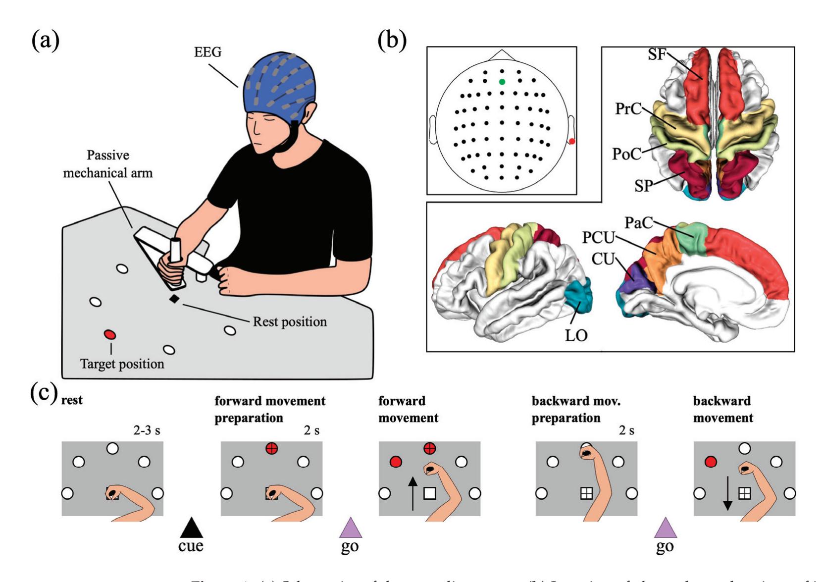
**Figure 1.** (**a**) Schematics of the recording setup. (**b**) Location of electrodes and regions of interest (ROIs). The electrodes were placed according to the 10/10 system and the ROIs considered in this study were taken from the Desikan–Killiany atlas. The reference channel (right earlobe) is marked in red, while the ground channel (AFz) in green. The selected ROIs were the cuneus (CU) and lateral occipital (LO) cortices as occipital regions, the precuneus (PCU) and superior parietal (SP) cortices as parietal regions, the post-central gyrus (PoC), the precentral gyrus (PrC), and the paracentral lobule (PaC) as peri-central regions, and the superior frontal gyrus (SF) as frontal region. (**c**) Trial sequence. Each trial started with a rest interval (2–3 s, random) that ended once a cue signal (target LED turning on) was provided to the participant indicating the target position. Then, the participant started preparing the center-out reaching movement (forward movement) and started the movement only after 2 s, once the first go-signal was provided (neighbor LED turning on). Once they reached the target, the participant held the position for 2 s while all LEDs were turned off. Finally, the second go-signal was provided (same as for the forward movement), triggering the backward movement toward the rest position. The fixation cross is displayed for each interval; note that, in the first scheme of panel c (rest interval 2–3 s), the fixation cross (at the rest position) is not visible since covered by the participants' hand.
#### 2.3.1. EEG Pre-Processing
The pre-processing consists of the following steps:
- i. Linear detrending of signals belonging to each recording block.
- ii. Band-pass filtering between 1 and 60 Hz and notch filtering at 50 Hz of signals belonging to each recording block. Notch filtering was applied also offline since visualization of the power spectral density of the recorded EEG signals evidenced insufficient attenuation of the power line noise by the notch filter applied during recording.
- iii. Identification of bad channels within signals of each recording block via random sample consensus method (RANSAC) [36].
- iv. Concatenation of electrode signals across recording blocks.
*Sensors* **2023**, *23*, 3530
- v. Removal of channels that were labelled as bad (step iii) at least in one recording block (3 ± 2 channels per subject removed, m ± std, ranging from 0 to 8).
- vi. Removal of artifacts (ocular, muscular, heart, and channel noise) via independent component analysis (ICA) via visual inspection of the components. ICA was computed using the extended Infomax algorithm [37,38] which estimates mixed sub-Gaussian and super-Gaussian sources. Across subjects, 31 independent components were removed, on average (ranging from 25 to 39). This relatively large number of removed ICs derives from the long-lasting recording (3750 s overall, obtained by concatenating 6 blocks) and on the type of performed task. Indeed, tasks involving motor activities are more prone to create isolated non-stereotypic artifacts (such as electrode pops, or complex movement artifacts) that are extracted in separated ICs and that add to the classical ICs separating stereotypic artifactual activity such as blinking, eye-movements, and heartbeat. We visually explored each IC (its time pattern, power spectral density, and topological map) carefully before removing it, in an effort to minimize the removal of potentially useful activity.
- vii. Spherical spline interpolation of the bad channels removed in step v.
- viii. Epoching into 4 s-length trials, starting 1 s before and ending 3 s after the presentation of the cue-signal, i.e., after the target LED to reach turned on. Thus, trials were defined from −1 s to 3 s, where 0 s corresponds to the onset of the cue-signal (corresponding to the black triangle in Figure 1c).
- ix. Baseline correction of each trial, by removing the mean value computed over the rest interval from −1 s to 0 s, channel by channel.
- x. Common average re-referencing.
All pre-processing steps were performed in Python using custom scripts and the functionalities of MNE Python library (version 1.2.2) [39] for implementing step vi.
#### 2.3.2. Cortical Activity Reconstruction and Computation of Activity within Regions of Interest (ROIs)
Sensor-space signals (scalp signals) were transformed into source-space signals (cortical signals) using MNE Python library (version 1.2.2) [39]. A template head anatomy was adopted using the FSaverage template, with the source space restricted to the cortex and discretized into 20,484 vertices. The forward problem [40] was solved via the boundary element method, applying MNE default parameters. The inverse problem [41] was solved using eLORETA (exact Low-Resolution Electromagnetic Tomography) [42] with MNE default parameters, with identity noise covariance matrix, and with the dipole source orientation constrained to be perpendicular to the cortex, resulting in one source signal per cortical vertex (i.e., 20,484 source signals).
The whole cortical surface was parcellated into 68 regions according to the Desikan– Killiany atlas [43], and we selected 8 regions of interest (ROIs) per hemisphere (16 in total) for our analysis. The selection of the ROIs was based on a priori information, considering the regions reported in the literature as most involved in motor planning and control during reaching movements [15,44,45]. The selected ROIs (see Figure 1b) included:
- i. The cuneus (CU) and the lateral occipital cortex (LO), located in the occipital lobe; they mainly have visual functions.
- ii. The precuneus (PCU) and the superior parietal lobule (SP), located in the posterior parietal cortex; they have associative (mainly visuomotor) functions, and their activations has been specifically associated to planning and execution of reaching movements [29].
- iii. The post-central gyrus (PoC), the precentral gyrus (PrC), and the paracentral lobule (PaC), located in the peri-central part of the cortex. They include the somatosensory cortex (PoC), the primary motor, premotor, and supplementary motor areas (PrC and PaC), and overall are denoted as sensorimotor ROIs.
- iv. The superior frontal gyrus (SF), located in the frontal region and implicated in high-level motor control functions [46].
253
*Sensors* **2023**, *23*, 3530
For each trial, a single waveform representative of the neural activity of each ROI was derived, by averaging all signals of the vertices belonging to that ROI. To avoid cancelling out the activity in case of many vertices in the ROI with dipole orientations in opposite directions, the signs of source signals that were not oriented as the "dominant direction" were flipped before averaging, as performed in Ghumare et al. [47]. The dominant direction was the first principal direction of all dipole orientations within the ROI. This sign flip procedure is adopted by Brainstorm toolbox [48] when using constrained dipole orientations.
### 2.3.3. Cortical Event-Related Spectral Perturbation
For each subject, each trial, and each ROI, the cortical event-related spectral perturbation (ERSP) were obtained based on the continuous wavelet transform of the cortical signal representative of that ROI using complex Morlet wavelet as basis function. Specifically, 'cmor1.5-1.0 was used as mother wavelet, with the first parameter denoting the bandwidth and the second parameter the normalized center frequency (normalized by the sampling period) [49]. Therefore, the mother wavelet had center frequency of 512 Hz with 4 oscillations (scales from 64 to 42 for alpha band, and from 42 to 16 for beta band). The wavelet transform coefficients were squared to obtain time-frequency power representations. Then, for each subject and each ROI, these representations were averaged across trials, separately for each of the 5 target positions, and normalized using the rest interval between −1 and 0 s as baseline (see Grandchamp et al. [50]). Specifically, for each frequency, the average power value between −1 and 0 s was computed, obtaining the average baseline power frequency by frequency. Then, the *ERSP* was computed as the difference between the power at each time-frequency point and the average baseline power at the same frequency, divided by this same average baseline power (thus, *ERSP* expresses the difference with respect to the baseline in percentage of the baseline).
Subsequently, for each subject and each ROI, the *ERSP* was averaged over the alpha band (8–13 Hz) and beta band (13–30 Hz), obtaining *alpha-ERSP* and *beta-ERSP*. We performed preliminary analyses by testing differences in *alpha-ERSP* and in *beta-ERSP* across different targets via permutation cluster tests [51] between each possible pair of targets, corrected for multiple comparisons via Benjamini–Hochberg [52] false discovery rate for each band. As no significant difference was found (*p* > 0.05), *alpha-ERSP* and *beta-ERSP* were also averaged across targets. Lastly, the time interval between the cue-signal and the go-signal was divided into two non-overlapped 1 s-length windows, i.e., from 0 to 1 s (early post-cue window) and from 1 to 2 s (late post-cue window, hereafter referred as *post-cuelate*). Then, we averaged the *alpha-ERSP* and *beta-ERSP* over the late post-cue window, obtaining the *post-cuelate alpha-ERSP* and *post-cuelate beta-ERSP*, which were assumed as mainly representative of the alpha and beta perturbations related to reaching movement preparation. The choice of considering this window is justified since the ERSPs in the early post-cue window were strongly affected by the visual evoked potential elicited by the lighting of the target LED.
This analysis was performed using custom Python scripts and the Python library PyWavelets [53] (version 1.4.1).
#### 2.3.4. Cortical Functional Connectivity and Degree Centralities (in Degree, out Degree)
For each subject, directional influences between ROIs in alpha and beta bands were estimated by computing pairwise Granger causality (GC) [54] in the frequency domain. Denoting with *xi*[*n*] and *xj*[*n*] two time series, here corresponding to the cortical signals representative of the i-th and j-th ROI (see Section 2.3.2), the system *xi*[*n*]; *xj*[*n*] can be represented using a bivariate autoregressive model with order *p* (*p* = 30 in this study, as we already adopted in previous studies, e.g., in Magosso et al. [55]). By Fourier-transforming this time-domain representation, a spectral representation is obtained. Then, the power spectrum of each time series (e.g., *xi*[*n*]) can be computed according to Geweke [56] and decomposed into an intrinsic term and a causal term, the latter being the term predicted by the other time series (e.g., *xj*[*n*]). The spectral GC from the j-th to the i-th ROI at each
254
*Sensors* **2023**, *23*, 3530
frequency *f* , *GCj*→*i*(*f*), is defined as the log of the ratio between the total power of *xi*[*n*] at *f* and the difference between the total power of *xi*[*n*] at *f* and the causal power exerted by *xj*[*n*] onto *xi*[*n*] at *f* . Thus, the quantity *GCj*→*i*(*f*) increases as the causal power increases. At each frequency *f* , the spectral GC is represented by a non-symmetric matrix with shape *NROI*×*NROI* (*NROI* = 16 in this study), with the off-diagonal ji-th value quantifying the directional influence from the j-th ROI to the i-th ROI at that frequency (*GCj*→*i*(*f*)).
Spectral GC was computed separately within two different 1 s-length windows, i.e., the baseline (rest) window from −1 to 0 s and the late post-cue window (reaching movement preparation, *post-cuelate*) from 1 to 2 s. The window from 0 to 1 s was neglected since it was strongly influenced by the transient due to the visual event related potential, elicited by the cue-signal. Still, to compensate for residual non-stationarities that might occur also in the considered windows in case of non-complete exhaustion of the evoked potential in the first post-cue second, the evoked potential was removed from each trial [57]. Rest windows and movement preparation windows were concatenated across trials, and spectral Granger causality was computed over the concatenated trials, thus estimating directional influences between ROIs across all trials in the two conditions. *Alpha*-GC and *beta-GC* were computed by averaging together the values of the GC spectrum belonging to alpha and beta bands, separately in the baseline and late post-cue conditions, resulting in 4 total connectivity matrices (*A* ∈ R*NROI*×*NROI* ) per subject (*baseline alpha-GC*, *baseline beta-GC*, *postcuelate alpha-GC*, *post-cuelate beta GC*). Furthermore, each connectivity matrix was normalized such that the sum of all off-diagonal connectivity values was 1 (∼ *A* = *A*/∑*i*,*j*;*i*=*j Aij*), thus emphasizing how much each connectivity value contributed to the overall connectivity across the selected ROIs as performed in [20].
Finally, indices derived from the graph theory were used to better understand changes in the topology of the brain connectivity network between baseline (rest) and late post-cue (movement preparation) conditions. Indeed, each matrix containing the connections values between the ROIs can be represented as a weighted directed graph, where each node corresponds to an ROI and the weight of each directed edge corresponds to the connection value. We computed two centrality indices, taking into account the direction of connections: the *in degree*—i.e., the sum of connectivity values entering into each ROI (quantifying the overall connectivity inflow)—and the *out degree*—i.e., the sum of connectivity values departing from each ROI (quantifying the overall connectivity outflow). The two indices were computed for each connectivity matrix, i.e., for each band (alpha and beta) and each condition (*baseline*, *post-cuelate*).
This analysis was performed using custom Python scripts, replicating the functions of the Brainstorm toolbox [48] (version 3.221212) that compute spectral Granger causality.
### 2.4. Statistical Analyses
The following tests were conducted:
- i. For all 16 ROIs, *post-cuelate alpha ERSP* and *post-cuelate beta ERSP* were compared to 0 (corresponding to the average baseline value after normalization), using Wilcoxon signed-rank tests. This comparison was performed to identify ROIs with a different ERSP during movement preparation compared to rest, separately for alpha and beta (16 test for each band). To correct for multiple tests, false discovery rate correction at *α* = 0.05 was applied, using the Benjamini–Hochberg procedure [52].
- ii. For all pairs of homologous ROIs, *post-cuelate alpha ERSP* and *post-cuelate beta ERSP* were compared between left and right ROIs using Wilcoxon signed-rank tests. This comparison was applied to identify ROIs with a lateralization in the spectral perturbations, separately for alpha and beta (8 tests, for each band). To correct for multiple tests, false discovery rate correction at *α* = 0.05 was applied, using the Benjamini–Hochberg procedure [52].
- iii. *Alpha-GC* and *beta-GC* were compared between *post-cuelate* and *baseline* using permutation tests (5000 permutations) [51]. This was performed to identify connections between ROIs that resulted in significantly differences during movement prepa-
255
*Sensors* **2023**, *23*, 3530
- ration compared to rest, separately for alpha and beta (16\*15 = 240 tests for each band).
- iv. For all ROIs, *in degree* and *out degree* in each band were compared between *postcuelate* and *baseline* using Wilcoxon signed-rank tests. This was performed to identify ROIs with a different inflow or outflow during movement preparation compared to rest, separately for alpha and beta (16 tests for each band and centrality index). To correct for multiple tests, false discovery rate correction at *α* = 0.05 was applied, using the Benjamini–Hochberg procedure [52].
#### 3. Results
### 3.1. Cortical Event-Related Spectral Perturbation
The grand average *ERSP* for each ROI is reported in Figure 2. A strong ERS is evident, spanning from the theta band (4–8 Hz) to the low beta band, associated to the visual evoked potential elicited by the cue-signal and go-signal (LED turning on). The ERS extinguished approximately 500 ms after each stimulus onset denoted by the black (cue) and purple (go) triangle in Figure 2. As expected, the ERS resulted more pronounced in visual (LO, CU) and visuomotor ROIs (SP, PCU) compared to the other ROIs, due to the visual nature of the stimuli. Furthermore, a clear ERD can be observed during the movement preparation period, in particular from 0.5–0.6 s to 2 s and during movement too, i.e., after the go-signal (from 2 to 3 s). The ERD involves both alpha and beta bands in the visual (LO, CU) and visuomotor ROIs (SP, PCU), and especially the beta band in the sensorimotor ROIs (PoC, PrC, PaC). Finally, the most frontal ROI included in the analysis (SF) showed less ERD compared to other ROIs.
By averaging the ERSPs represented in Figure 2 over the alpha and beta bands, the *alpha-ERSPs* and *beta-ERSPs* were computed and are reported in Figure 3, to better visualize the ERSP temporal dynamic in these frequency ranges. Concerning *alpha-ERSPs* (Figure 3a), the following observations can be made with a focus on the movement preparation period (i.e., 0–2 s). In agreement with Figure 2, a strong ERS was elicited by the cue-stimulus, especially in visual (LO and CU) and visuomotor ROIs (PCU and SP). In the other ROIs, ERS was smaller. Cue-related ERS was followed by ERD (except than in SF), especially in the late post-cue interval (1–2 s). In this interval, ERD was approximately constant in visual and visuomotor ROIs, while it kept gradually increasing (from approximately 0 to −15%) in the sensorimotor ROIs (PoC, PrC, PaC).
Concerning *beta-ERSPs* (Figure 3b) in the same period (0–2 s), similar observations held in visual and visuomotor ROIs, with evident ERS produced by the cue stimulus followed by ERD, in particular in the late post-cue interval. In the other ROIs, only ERD occurred. Furthermore, the pattern of beta-ERD exhibited some differences compared to alpha-ERD. In the sensorimotor ROIs, the gradual increase in post-cue ERD was more pronounced in the beta band (up to −25%) than in the alpha band. Furthermore, in several ROIs, beta-ERD showed appreciable differences between the two hemispheres, with the contralateral hemisphere reaching lower ERD values (up to −25%) compared to the ipsilateral hemisphere (up to −12%). Finally, while in visual ROIs alpha-ERD was almost constant during the late post-cue interval, in the same interval, beta-ERD in the visual ROIs tended to decrease (i.e., assumed less negative values), showing a partial return towards baseline value (i.e., 0%).
Of course, as the reported representations refer only to epochs including rest (from −1 to 0 s), reaching preparation (from 0 to 2 s), and at least part of center-out reaching execution (from 2 to 3 s), the rebound of the ERSP recovering the resting condition value before the start of the new trial (i.e., 0) is not evident from these figures. Thus, Supplementary Figure S1 displays the alpha- and beta-ERSP over a longer epoch for Cz, an electrode site representative of the motor-related response, showing that the ERSP rebounded once the subject returned to the rest position (backward movement completed), and confirming that resting condition is recovered before the beginning of a new trial.
256
*Sensors* **2023**, *23*, 3530
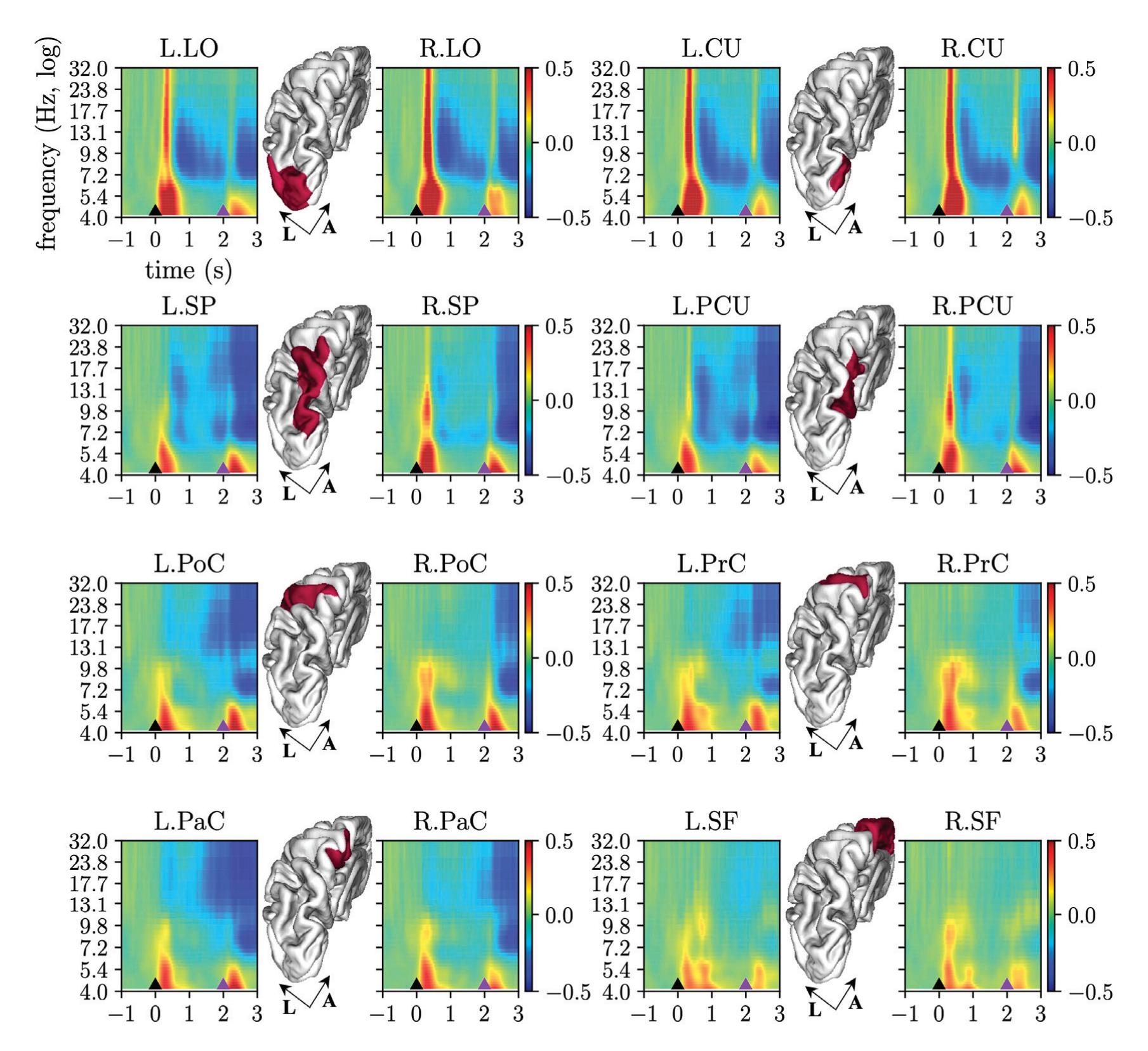
**Figure 2.** Event-related spectral perturbations (ERSPs). The grand-average ERSP is reported for each selected ROI of the left (label prefix "L.") and right (label prefix "R.") hemisphere. The small black and purple triangles at the bottom of each plot mark the time associated with the cue onset and go onset of the center-out reaching movement, respectively. To increase readability, x- and y-labels are reported only for the first plot. The position of each ROI is also visualized, limited to the left hemisphere, highlighted in red in the 3-D view of the cortex (A: anterior, L: lateral).
Figure 4 reports the alpha- and beta-ERSP averaged over the late post-cue interval (*post-cuelate alpha-ERSP* and *post-cuelate beta-ERSP*), and the results of the statistical analyses. Significant ERD (*p* < 0.05) during movement preparation was obtained for all ROIs compared to rest in the beta band, and for visual and visuomotor ROIs in the alpha band. Furthermore, ERD results were significantly (*p* < 0.05) stronger in the contralateral hemisphere in the beta band (but not in the alpha band) for all ROIs except LO and PCU, with higher significance for sensorimotor ROIs (*p* < 0.005 for PoC and PaC, *p* < 0.01 for PrC).
257
*Sensors* **2023**, *23*, 3530
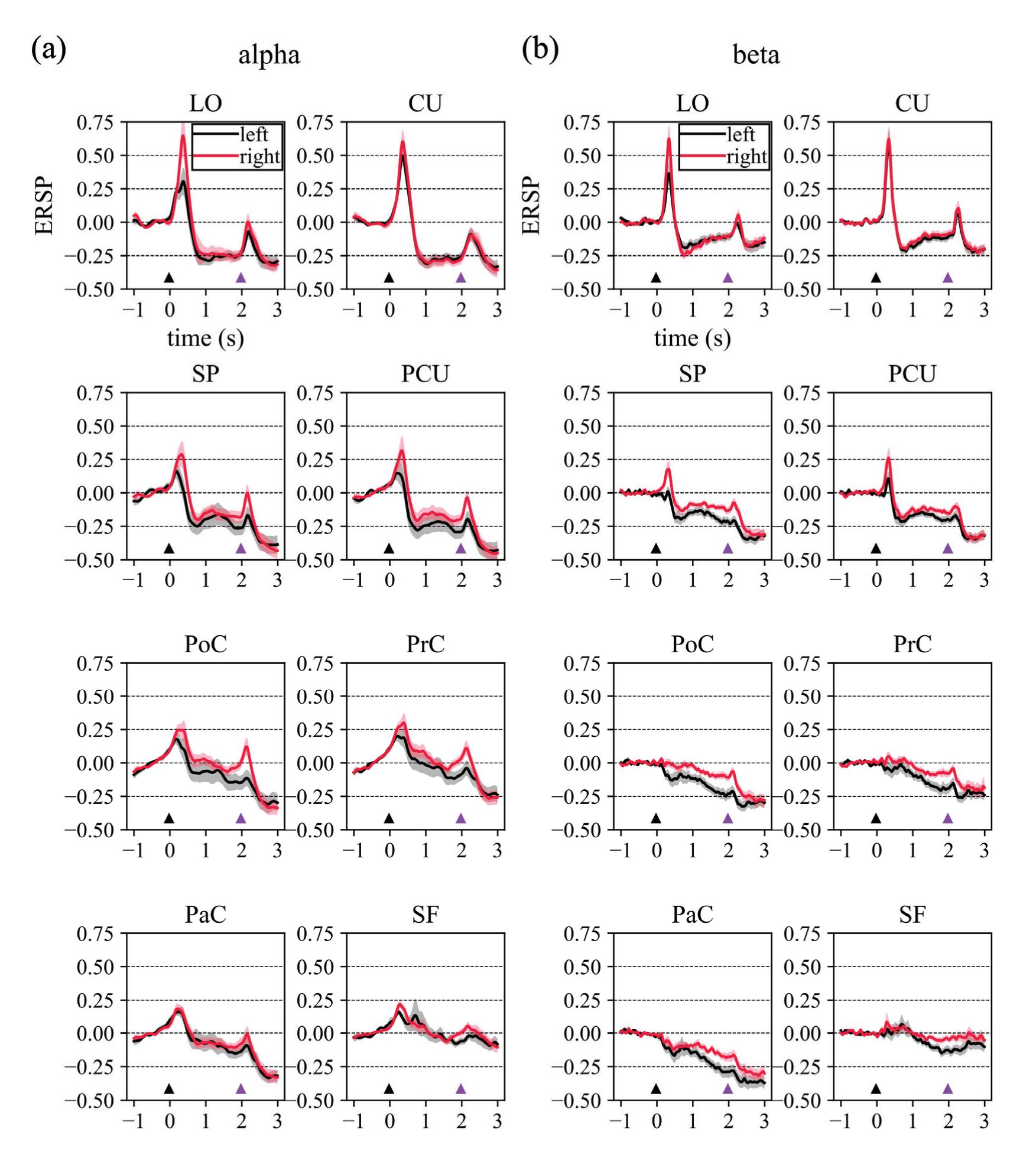
**Figure 3.** Alpha (**a**) and beta (**b**) event-related spectral perturbations (ERSPs). Here, the ERSPs reported in Figure 2 were averaged within alpha and beta bands and visualized as a function of time. The grand-average alpha-ERSP and beta-ERSP is reported for each selected ROI of the left (black thick lines) and right (red thick lines) hemisphere. Shaded areas denote the standard error of the mean across subjects (in grey for the left ROI, in red for the right ROI). The small black and purple triangles shown at the bottom of each plot mark the time associated with the cue onset and go onset of the center-out reaching movement, respectively. Note that in this figure, to increase the readability, x- and y-labels are reported only for the first plot.
258
*Sensors* **2023**, *23*, 3530
### 3.2. Cortical Functional Connectivity and in Degree and out Degree Indices
The connections that were significantly higher (in red) or lower (in blue) in the late post-cue interval compared to baseline are displayed in Figure 5, separately for the alpha band (left panel) and beta band (right panel). Decreased alpha-band connectivity was mainly localized posteriorly, involving bilateral visual (occipital) and visuomotor (parietal) ROIs, but also with a left-lateralized involvement of sensorimotor regions (L.PrC). Increased alpha-band connections were mainly directed from left to right, especially toward right sensorimotor regions. As to the beta band, left ROIs (in particular visuomotor and sensorimotor) exhibited decreased connections, both entering and exiting, while right ROIs overall showed increased entering and exiting beta-band connections.
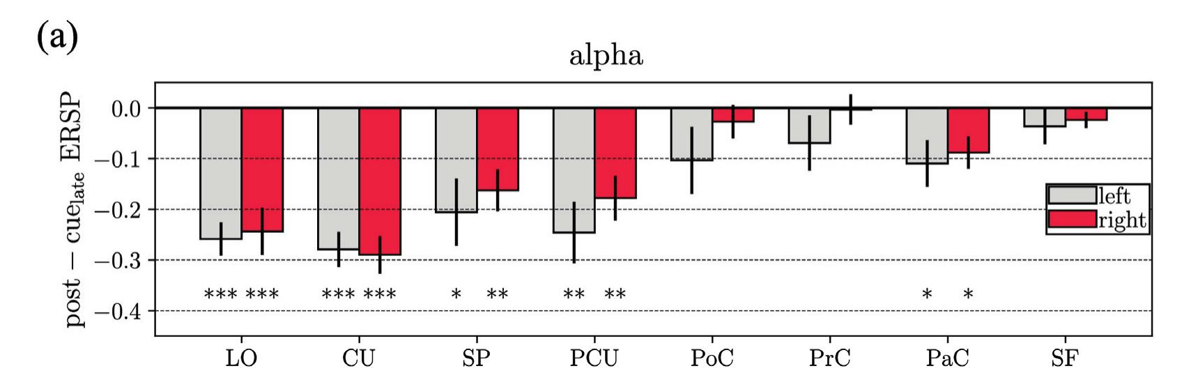
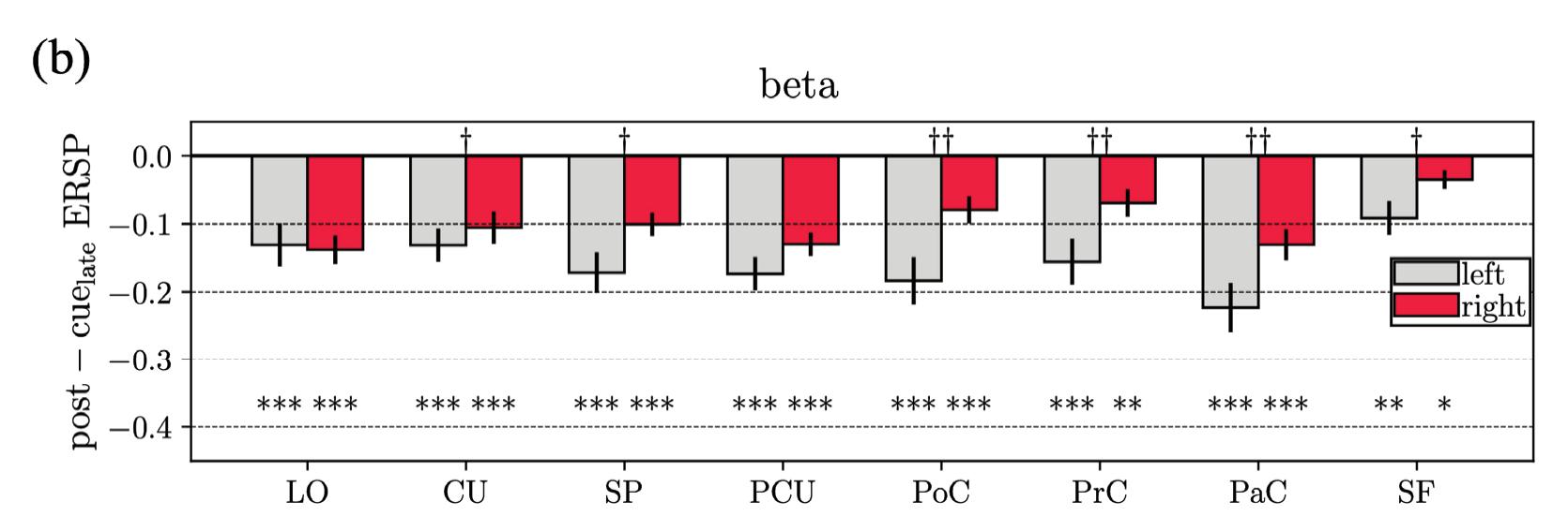
**Figure 4.** Alpha (**a**) and beta (**b**) event-related spectral perturbations (ERSPs) during reaching movement preparation. Here, the alpha-ERSP and beta-ERSP reported in Figure 3 were averaged within the second half of the movement preparation interval of the center-out reaching movement (i.e., from 1 to 2 s with respect to cue onset). These values are also referred to in the manuscript as *post-cuelate alpha-ERSP* and *post-cuelate beta-ERSP*. In each panel, for each ROI (grey: left ROI, red: right ROI) the bar height denotes the mean value across the subject and the error bar the standard error of the mean. Results of the performed statistical analyses are reported too. Specifically, symbols \* (reported at the bottom of each panel) denote ERSPs significantly different compared to the baseline (\* *p* < 0.05, \*\* *p* < 0.01, \*\*\* *p* < 0.001). Symbols † (reported at the top of each panel) denote ROIs with significantly different ERSP between the left and right hemisphere († *p* < 0.05, †† *p* < 0.01).
Figures 6a and 7a report the ROIs that exhibited significantly different in degrees (left) and out degrees (right) for the alpha and beta bands, respectively, when comparing late post-cue interval to baseline. Each bar plot in Figures 6b and 7b shows, for a selected ROI, the difference (late post-cue minus baseline) in the connections entering into the selected ROI from each other ROI, or exiting from the selected ROI towards each other ROI. The
259
*Sensors* **2023**, *23*, 3530
shown differences highlight the ROIs contributing more to the in degree or out degree of the selected ROI (significant differences are indicated by grey bars).
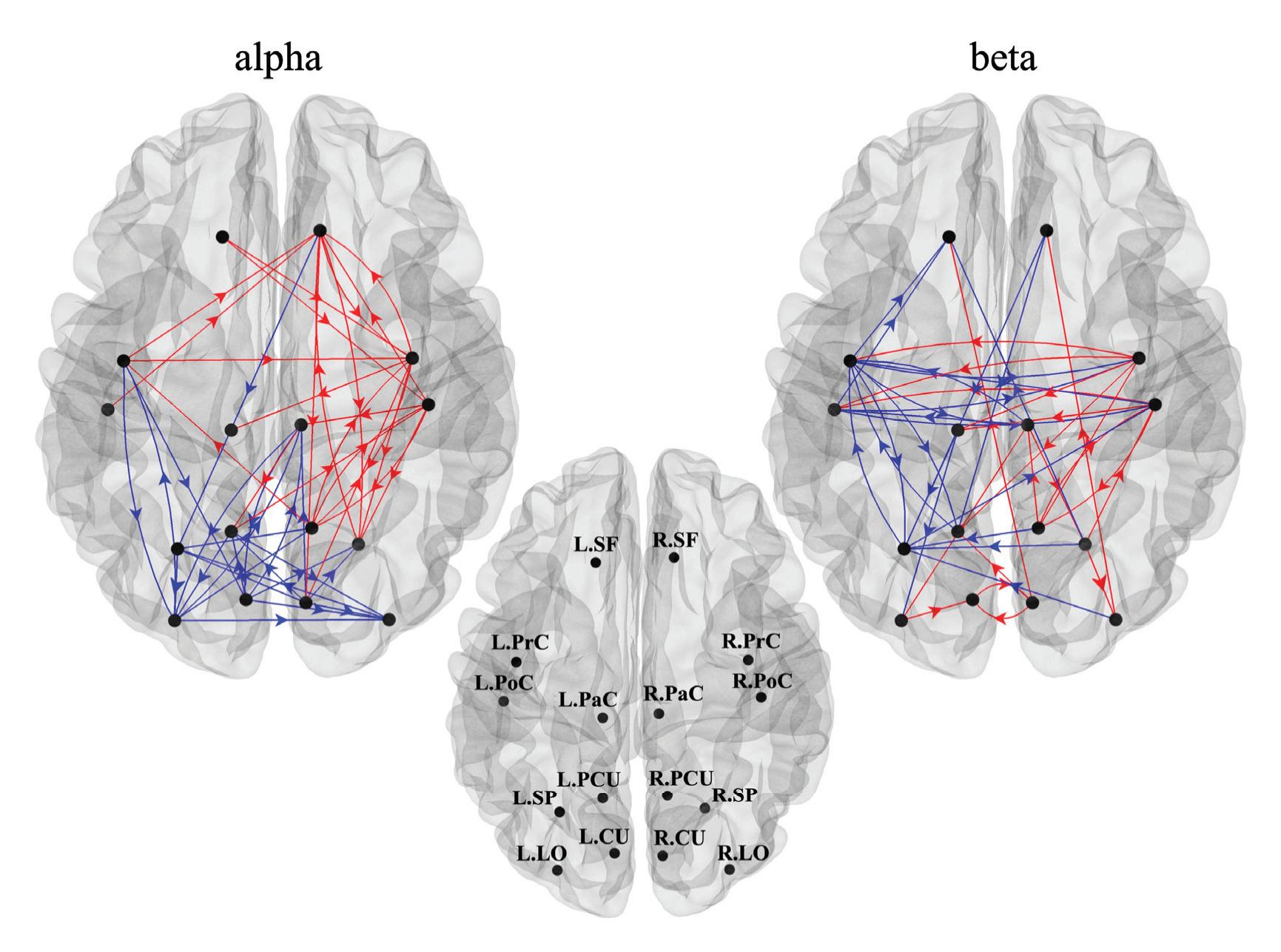
**Figure 5.** Directed connections between ROIs—as measured by the spectral Granger causality—that resulted significantly higher (in red) or lower (in blue) during reaching movement preparation compared to rest, in alpha (**left**) and beta (**right**) bands. To improve readability, ROI labels are displayed on the cortex in the middle panel, separately from the other panels.
As to the alpha band (Figure 6), the late post-cue interval was characterized by a significantly lower alpha-inflow in bilateral visual ROIs (L.LO and R.LO), a significantly higher alpha-inflow in ipsilateral frontal ROI (R.SF) and in ipsilateral sensorimotor ROIs (R.PrC and R.PoC). The latter was mainly mediated by ipsilateral visual and visuomotor ROIs (R.CU and R.PCU), by a contralateral sensorimotor ROI (L.PrC), and by the bilateral frontal ROIs (L.SF and R.SF). Moreover, the same ipsilateral sensorimotor areas (R.PrC and R.PoC) that were shown to be higher in degree also exhibited a significantly increased alpha-outflow mainly towards other areas in the same hemisphere (among them R.SP, R.PCU, R.SF).
As to the beta band (Figure 7), some visual ROIs (L.CU and R.CU) exhibited significantly higher beta-inflow and beta-outflow. The contralateral visuomotor ROI L.SP was characterized by a significantly decreased beta-inflow, especially from sensorimotor ROIs in the same hemisphere (L.PrC and L.PaC). Indeed, the latter ROIs, together with L.PoC, had decreased beta-outflow not only towards L.SP but, interestingly, also towards ipsilateral sensorimotor ROIs (R.PrC and R.PoC).
260
*Sensors* **2023**, *23*, 3530
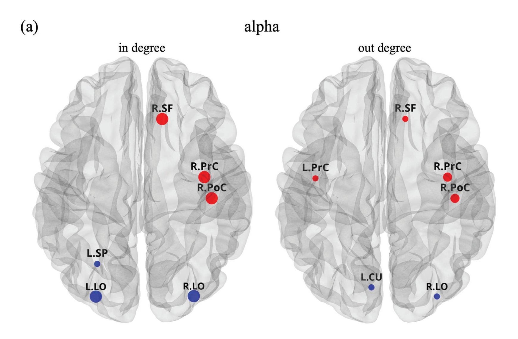
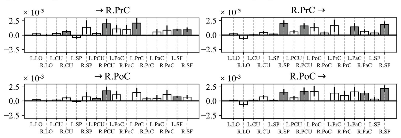
**Figure 6.** (**a**) ROIs with a significantly different in degree (left panel) and out degree (right panel) during reaching movement preparation compared to rest in the alpha band. Circle size reflects the strength of the significance (small: *p* < 0.05, medium *p* < 0.01, large: *p* < 0.001); red/blue circles denote an increased/decreased measure (in degree or out degree) during movement preparation compared to rest. (**b**) Each bar plot shows, for a selected ROI among the ones in panel a, the difference in the connections (movement preparation—rest) entering in the selected ROI from all other ROIs or exiting from the selected ROIs towards all other ROIs. The bar height denotes the mean value across the subjects and the black line the standard error of the mean. Significant differences are marked via grey bars.
261
*Sensors* **2023**, *23*, 3530
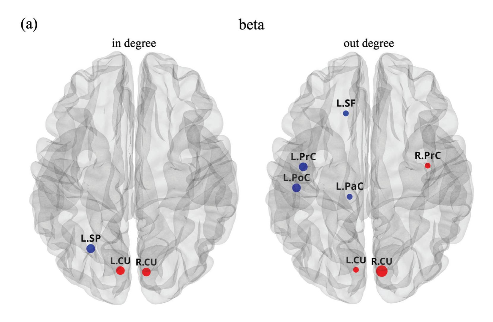
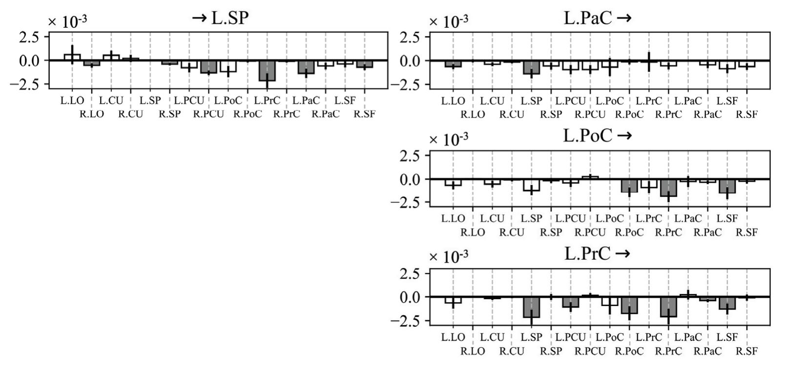
**Figure 7.** (**a**) ROIs with a significantly different in degree (left panel) and out degree (right panel) during reaching movement preparation compared to rest in the beta band. (**b**) Each bar plot shows, for a selected ROI among the ones in panel a, the difference in the connections (movement preparation rest) entering in the selected ROI from all other ROIs or exiting from the selected ROIs towards all other ROIs. See the caption of Figure 6 for further details.
## 4. Discussion
This study investigates alpha and beta mechanisms related to the preparation of reaching movements by analyzing the cortical activity by means of event-related spectral perturbations, and the connectivity between regions by means of spectral Granger causality and graph analysis. The analysis of brain connectivity, either at rest or during a task, is 262
*Sensors* **2023**, *23*, 3530
today recognized as a fundamental tool to gain insights into how different brain regions work together (in a synergistic or antagonistic way) and exchange information to achieve behavior, and how this coordinated activity is disrupted in pathological states. Among the measures of connectivity, GC is a popular statistical method to analyze directed interactions in multivariate dynamical systems [58]. An attractive property of GC for brain connectivity investigation is its frequency domain formulation, eligible for the analysis of causal interactions in specific frequency bands and, thus, particularly relevant in the case of neuroelectric signals, extremely rich in oscillatory content. In the context of brain connectivity networks, graph theoretical approaches provide a powerful way to quantify the topological properties of the networks, inferring meaningful attributes that improve the understanding of connectivity patterns and of their functional roles [59].
The present study provides a novel contribution to the investigation of electromagnetic brain activity and connectivity in reaching tasks. To the best of our knowledge, this is the first time that directed connectivity and direction-sensitive indices derived from the graph theory, joined with ERSP analysis, are applied to investigate a large set of brain areas in the preparation phase of a reaching task, providing an enriched EEG characterization and interpretation of brain regions' activation and of their causal interactions during reaching movement preparation. Specifically, here, both ERSP and spectral GC were analyzed on the cortical activity reconstructed from the EEG while healthy subjects prepared a reaching movement compared to a rest condition.
### 4.1. Event-Related Spectral Perturbations
Reaching movement preparation was associated to alpha-ERD in visual and visuomotor ROIs (and only one sensorimotor ROI). Even though alpha-ERD exhibited slightly stronger results in the contralateral hemisphere (e.g., for SP and PCU in Figure 4), no significant differences were observed between hemispheres. It is worth noticing that this result held also without averaging together different targets, i.e., by performing the ERSP analysis within each single target, as reported in Supplementary Figure S2. From this figure, no significant inter-hemispheric difference in the alpha band was observed, widely across ROIs and targets, except only for the target located most rightwards, that showed a stronger alpha-ERD for the contralateral side in PrC and PoC. Alpha-ERD is likely associated to the goal-directed visuomotor nature of the task, involving both visuo-spatial attention and the processing of spatial information to guide the hand to the proper position accurately (i.e., location of the target LED). As to the beta band, widespread beta-ERD was observed, stronger in sensorimotor and visuomotor ROIs, and significantly higher in the contralateral hemisphere in particular for the sensorimotor ROIs (this result held also within each target, see Supplementary Figure S3). These results on alpha- and beta-ERD agree with the study of Wang et al. [10], showing that during visually-cued movement preparation (even though finger movement and not reaching movement was analyzed), alpha-ERD was localized more posteriorly, while beta-ERD was more widespread and more lateralized. Considerations also come by looking at the alpha- and beta-ERSP dynamic in Figure 3. The visuomotor and mainly the sensorimotor ROIs exhibited time-increasing ERD (i.e., time-increasing disinhibition) in the alpha band and especially the beta band throughout the movement preparation period, with ERD further increasing during movement execution. This suggests a progressively growing engagement of sensorimotor ROIs during the entire trial, from movement preparation to execution. The same did not hold for visual ROIs (LO and CU). Indeed, after the transient related to visual-evoked potential, visual ROIs exhibited a constant alpha-band disinhibition in the preparation phase, suggesting a sustained visuo-spatial attention while preparing the action. Conversely, these ROIs tended to rapidly deactivate (i.e., ERSP tended to partially return towards 0) in the beta band, indicating a more marginal role in motor planning. Differences in alpha- and beta-ERD suggested that these rhythms are to some extent independent and with distinct functional relevance. Indeed, while the suppression of beta oscillations is tied to the activation of
263
*Sensors* **2023**, *23*, 3530
neuronal populations involved in movement, the suppression of alpha oscillations also reflects visual information processing and cognitive processing related to attention [60].
### 4.2. Connectivity Network and Centrality Indices
Causal influences between ROIs were analyzed via spectral GC and differences in connectivity network were assessed between reaching movement preparation and rest. In degree and out degree centrality indices were computed, quantifying overall connectivity inflow and outflow for each ROI, and were used to identify the ROIs that significantly exhibited changes in inward and outward connections during movement preparation compared to rest. It is worth noticing that, despite these differences being quantified by aggregating the information across reaching targets, the result was not driven by a small subset of targets, as the obtained differences were similar across targets (see Supplementary Figures S4–S7).
As to alpha-band connectivity, decreased interactions were mainly in visuomotor and visual regions, and were probably linked to the reduced amplitude of alpha oscillations in these ROIs (see alpha-ERD in Figure 2) and related to visual information processing (as decreased connectivity values can be related to desynchronization [35]). Interestingly, our results indicate a prevalent anterior-to-posterior direction of decreased alpha connections (from parietal to occipital and also from front-central to parietal and occipital regions), and with bilateral LO that most showed reduced alpha inflow. Previous studies have reported top-down modulatory influences in the alpha band from higher-level frontal and parietal areas to the lower-level visual cortex, as a mechanism for controlling visuo-spatial attention via facilitation (decreased alpha-band influences) and inhibition (increased alpha-band influences) [61,62]. Our findings appear in line with this hypothesis, with decreased inflow in the early visual cortex facilitating visual processing of stimuli for goal-directed movement. Decreased anterior-to-posterior alpha connectivity was accompanied by increased left-toright alpha connections, and significantly higher alpha-inflow in ipsilateral sensorimotor ROIs. Importantly, the latter was also mediated by a contralateral sensorimotor ROI (L.PrC, see Figure 6b-left). Considering the inhibitory role of alpha rhythm, these results agree with previous evidence of inhibitory inter-hemispheric interactions between sensorimotor cortices [14] (concurring at facilitating the movement) that may be functionally implemented via alpha oscillations [10]. Furthermore, the inhibition of ipsilateral sensorimotor ROIs (R.PrC and R.PoC) was also exerted by a top-down mechanism operated by the two frontal ROIs (L.SF and R.SF, see Figure 6b-left), suggesting that top-down alpha influences from higher level areas can also be implicated in modulating (inhibiting or facilitating) motorrelated processing other than sensory processing. Lastly, ipsilateral sensorimotor ROIs were also characterized by an increased alpha-outflow, mainly confined in the ipsilateral hemisphere (see Figure 6b-right), thus potentially contributing to further spreading and sustaining the inhibition in the ipsilateral hemisphere.
As to beta-band connectivity, a first notable result is the significantly higher betainflow and beta-outflow observed in visual ROIs (L.CU and R.CU). This might be related to ERD in the beta band that tended to reduce in the visual areas (ERSP tending to return closer to 0, Figure 3b upper panel) and that may be interpreted as an early disengagement of visual cortices from motor processing. Indeed, while visuomotor and sensorimotor ROIs likely contribute to motor-related processing in a sustained or increasing manner during the movement preparation period (as supported by their constant or increasing ERD dynamic, see Figure 3), it seems reasonable that visual cortices deactivate earlier. The second notable result is the significantly lower beta-outflow observed in contralateral sensorimotor ROIs (L.PrC, L.PoC, L.PaC) that had the main effect of significantly reducing beta-inflow in contralateral visuomotor ROIs (L.SP, Figure 7b-right). Based on this result, contralateral sensorimotor ROIs might act as hubs for beta-band desynchronization among movement-related regions, and such decoupling may represent a mechanism to interrupt the maintenance of the current motor output and favor regions to be engaged in the impending movement. Indeed, beta-band synchronization has been hypothesized to
264
*Sensors* **2023**, *23*, 3530
promote maintenance of the current sensorimotor state, while compromising the neural processing of new movements [63]. In this regard, it is also interesting to note that the two hemispheres are characterized by opposite changes in beta-band connections, with mainly increased beta-band connections entering and exiting from the ROIs in the ipsilateral hemisphere, as opposed to the contralateral hemisphere. This may indicate a coordinated beta-band competition between the two hemispheres, functionally relevant for performing unilateral movements.
As highlighted by our results, by analyzing the EEG via complementary investigations in the frequency domain (via ERSP and spectral GC, using also indices derived from graph theory), an enriched characterization of the preparation of reaching movements was provided. Overall, these findings substantiate the idea of the presence of different mechanisms during movement preparation operated by alpha and beta rhythms, comprising an alpha-mediated inhibition mechanism on the ipsilateral sensorimotor areas, and a betamediated disinhibition mechanism of the contralateral visuomotor and sensorimotor areas. Furthermore, alpha oscillations emerge as a general mechanism for inhibiting processing in task-irrelevant regions (alpha increase) and facilitating processing in task-relevant regions (alpha decrease), involving both motor and sensory regions. Conversely, beta-band desynchronization appears as a more motor-specific disinhibition mechanism; indeed, despite the widespread beta-ERD involving all regions, connectivity analysis reveals spatially specific differences in beta-band interactions where visual areas (although actively involved in sensory processing during the task) and also ipsilateral motor-related areas were characterized by beta-band connectivity increase. The present study not only contributes to expanding the neurophysiological description of motor-related mechanisms but may also have clinical and practical implications. For example, connectivity appears as a measure able to capture more subtle changes in brain functioning; thus, brain connectivity may provide markers of neuromotor disorders more sensitive to progression or improvement. Moreover, measures of connectivity have potential applications in motor-based brain–computer interfaces; indeed, motor states can be decoded exploiting artificial intelligence approaches not only by using scalp-level EEG [64,65], but also from features related to brain network connectivity [66]. Interestingly, the knowledge learned by these decoders could also be exploited to analyze, in a data-driven way, the most relevant interactions for a target variable under analysis [64,65,67–69] (e.g., a specific movement), by designing and applying explainable artificial intelligence approaches specific for functional connectivity analyses.
Of course, the present study has some limitations. First, our analyses were not conducted on the whole cortex parcellation but on a selection of ROIs known to be implicated in reaching movement preparation and control. However, other ROIs (not considered in the performed analyses) may also be involved, e.g., the right inferior frontal gyrus (R.IF), a region found to play a role in motor control via top-down inhibition of planned or ongoing action [70]. As complementary analyses, we also performed the same analyses conducted in this study for bilateral IF areas in Supplementary Figures S8 and S9. Here, the signal representative of L.IF and R.IF was obtained, for each hemisphere, by averaging the signals of the pars opercularis, pars orbitalis, and pars triangularis, since these three regions compose the inferior frontal gyrus in the Desikan–Killiany atlas, adopted in this study for cortex parcellation. As obtained for SF, IF (both left and right) had small and bilateral ERDs during movement preparation and was involved in the alpha-mediated top-down inhibition of the ipsilateral sensorimotor areas. Thus, future studies could benefit from considering the whole cortex parcellation to avoid missing potentially relevant ROIs. Furthermore, the selected ROIs were based on the Desikan–Killiany atlas, and some of them englobe large portions of the cortex. In particular, as concerning the sensorimotor areas, we did not specifically consider the primary motor cortex (M1), supplementary motor areas (SMA), and premotor cortex (PMC), which are small regions in the sensorimotor cortex, and deemed to be core motor areas, largely investigated in connectivity studies [23,34,35]. Rather, we preferred to consider larger areas (likely englobing the previous core areas) also due to the use of a template head model for cortical source estimation, rather than
265
*Sensors* **2023**, *23*, 3530
individual head models. The use of a template head model (which, however, is commonly adopted in the literature when individual brain MRIs are not available [71]), unavoidably leads to a reduction in spatial accuracy in source localization and spatial inaccuracy may have a greater effect when small areas consisting of a low number of voxels are selected. By considering the average behavior of larger areas, spatial inaccuracies may have a more tolerable impact. Another limitation is related to the adoption of a fixed and short time window for computing the spectral GC, i.e., 1 s windows for rest and 1 s windows for reaching preparation, concatenated across trials. Indeed, movement preparation is a dynamic process that could benefit from a dynamic description of connectivity between brain regions. Furthermore, more accurate results with parametric spectral GC are known to be obtained as the window length increases [58]. However, due to the trial-based nature of the experimental paradigm, the movement preparation phase was inherently limited. These aspects may be addressed in the near future by studying the dynamic of spectral GC via non-parametric methods.
#### 5. Conclusions
In conclusion, in this study, we investigated the frequency-specific changes in cortical activity and in directed connectivity evoked by the preparation of a reaching task within a network of task-related areas, spanning from occipital to parietal and fronto-central cortices.
Our results suggest that alpha and beta oscillations are functionally involved in the preparation of reaching movements in different ways. That is, beta mainly reflects the disinhibition of areas involved in movement, mainly contralateral visuomotor and sensorimotor areas, and concurs at coordinating the disinhibition among these areas. Alpha also reflects visual processing and visuo-spatial attention and concurs at mediating an inhibition mechanism (inter-hemispheric and top-down) of the ipsilateral sensorimotor areas (to facilitate the preparation of the unilateral upcoming movement) and the disinhibition of visual cortices (to facilitate visuo-spatial attention during preparation).
Overall, this study contributes to enriching the description of the neural mechanisms underlying reaching movement preparation in healthy subjects, for a better comprehension of the neurophysiological correlates. In prospective, this knowledge could be useful to analyze alterations occurring in pathology (e.g., stroke) and to improve diagnostic and therapeutic applications.
**Supplementary Materials:** The following supporting information can be downloaded at: https:// www.mdpi.com/article/10.3390/s23073530/s1|, Figure S1: Alpha (a) and beta (b) event-related spectral perturbations (ERSPs) at Cz considering a larger epoch (from −1 to 11 s respect to the cue-onset) than the one used in the main text (from −1 to 3 s). The epoch considered here includes the overall trial, i.e., both the forward and backward movement, from 0 to 10 s; an additional final second is displayed (from 10 to 11 s), reporting also the first second of the random inter-trial interval (ranging from 2–3 s randomly) of the subsequent trial. This analysis was performed to observe the ERSP dynamic for a longer period, checking for ERSP rebound towards rest values (i.e., towards 0). Here, ERSPs were computed at the scalp level using the same procedure as at source-level (see Section 2.3.3) and are visualized as a function of time (as reported in Figure 3 at the source-level). Black tick line denotes the grand-average alpha-ERSP in the left plot and the grand-average beta-ERSP in the right plot, and shaded grey area denotes the standard error of the mean across subjects. The small black and purple triangles shown at the bottom of each plot mark the time associated to the cue onset and go onset of movements, respectively. The first purple triangle refers to the go-onset for the forward movement, while the second one refers to the backward movement. Figure S2. Target-specific alpha event-related spectral perturbations (ERSPs) during reaching movement preparation (*post-cuelate* interval), in the different ROIs. Here, for each ROI, the alpha-ERSP was averaged within the second half of the movement preparation interval (from 1 to 2 s with respect to cue onset, i.e., *post-cuelate* interval), separately for each target to reach. For each target and each ROI (grey: left ROI, red: right ROI), the bar height denotes the mean value across the subject and the error bar the standard error of the mean. The black square represents the rest position of the hand; 266
*Sensors* **2023**, *23*, 3530
the bar plots are topologically arranged inside the page according to the target position they refer to. The same statistical analyses as the ones conducted to produce Figure 4 in the main text were performed here; however, instead of performing comparisons based on *post-cuelate* ERSP averaged across targets, the comparisons were performed separately for each target. Results of the performed statistical analyses are reported using symbols: symbols \* (at the bottom of each panel) denote ERSPs significantly different compared to baseline (\* *p* < 0.05, \*\* *p* < 0.01, \*\*\* *p* < 0.001); symbols † (at the top of each panel) denote ROIs with significantly different ERSP between the left and right hemisphere († *p* < 0.05, †† *p* < 0.01, ††† *p* < 0.001). Reported statistical results are corrected for multiple comparisons, with correction applied separately within each target. Note that significant inter-hemispheric difference was observed only in case of the most rightward target (bar plot at the bottom right), as to ROI PoC and PrC, with alpha-ERD significantly larger in the contralateral ROI than in the ipsilateral one. Figure S3. Target-specific beta event-related spectral perturbations (ERSPs) during reaching movement preparation (*post-cuelate* interval). Here, for each ROI, the beta-ERSP was averaged within the second half of the movement preparation interval (from 1 to 2 s with respect to cue onset, i.e., *post-cuelate* interval), separately for each target to reach. See the caption of Supplementary Figure S2 for further details. Note that significant inter-hemispheric difference was observed for several targets and ROIs (especially sensorimotor and visuomotor), with beta-ERD significantly larger in the contralateral ROI than in the ipsilateral one. This result is in agreement with results obtained collapsing together all targets (see Figure 4 in the main text). Figure S4. ROIs with a significantly different in degree between center-out reaching preparation and rest in the alpha band, separately for each target position. The black square represents the rest position and each in degree representation is topologically placed according to the target it refers to. The same statistical analysis as the one conducted to produce Figs. 6 and 7 in the main text was performed. However, instead of performing comparisons based on the connections averaged across targets, the comparisons were performed separately for each target. Circle size reflects the strength of the significance (small: *p* < 0.05, medium *p* < 0.01, large: *p* < 0.001); red/blue circles denote an increased/decreased measure (in degree or out degree) during movement preparation compared to rest. Figure S5. ROIs with a significantly different out degree between center-out reaching preparation and rest in the alpha band, separately for each target position. The black square represents the rest position. See the caption of Supplementary Figure S4 for further details. Figure S6. ROIs with a significantly different in degree between center-out reaching preparation and rest in the beta band, separately for each target position. The black square represents the rest position. See the caption of Supplementary Figure S4 for further details. Figure S7. ROIs with a significantly different out degree between center-out reaching preparation and rest in the beta band, separately for each target position. The black square represents the rest position. See the caption of Supplementary Figure S4 for further details. Figure S8. Alpha (a) and beta (b) event-related spectral perturbations (ERSPs) of the inferior frontal (IF) gyrus. The grand-average alpha-ERSP and beta-ERSP is reported for the left (black tick lines) and right (red tick lines) hemisphere. Shaded areas denote the standard error of the mean across subjects (in grey for the left ROI, in red for the right ROI). The small black and purple triangles shown at the bottom of each plot mark the time associated to the cue onset and go onset of the center-out reaching movement, respectively. Figure S9. Directed connections between ROIs—as measured by the spectral Granger causality—that resulted significantly higher (in red) or lower (in blue) during reaching movement preparation compared to rest, in alpha (left) and beta (right) bands. Here, also the inferior frontal (IF) gyrus is added to the set of ROIs considered in the study (thus, here, 18 ROIs in total are considered). To improve readability, ROI labels are displayed on the cortex in the middle panel, separately from the other panels.
**Author Contributions:** Conceptualization, E.M. and D.B.; Methodology, E.M., D.B., S.F. and M.C.B.; Software, D.B. and E.M.; Formal Analysis, D.B. and E.M.; Investigation, D.B. and M.C.B.; Data Curation, D.B and M.C.B.; Resources, E.M. and S.F.; Visualization, D.B. and E.M.; Supervision, E.M. and S.F.; Project Administration, E.M.; Writing—Original Draft Preparation, D.B. and E.M.; Writing— Review and Editing, S.F. and M.C.B. All authors have read and agreed to the published version of the manuscript.
**Funding:** Part of this study was funded by of the Italian Ministry of Education, Universities and Research (MIUR), within the 'Department of Excellence' project (years 2018–2022) of the Department of Electrical, Electronic and Information Engineering, University of Bologna. This work is also supported by #NEXTGENERATIONEU (NGEU) and funded by the Ministry of University and 267
*Sensors* **2023**, *23*, 3530
Research (MUR), National Recovery and Resilience Plan (NRRP), project MNESYS (PE0000006)—A Multiscale integrated approach to the study of the nervous system in health and disease (DN. 1553 11.10.2022).
**Institutional Review Board Statement:** The study was conducted according to the guidelines of the Declaration of Helsinki and approved by the Bioethics Committee of University of Bologna (protocol code: 61243, date of approval: 15 March 2021).
**Informed Consent Statement:** Written informed consent was obtained from all subjects involved in the study.
**Data Availability Statement:** The data presented in this study are available on request from the corresponding author.
**Acknowledgments:** The authors gratefully acknowledge Matteo Fraternali, Lorenzo Orsini, Annalisa Taddei, Gaia Sammarini, and Federico Piras, for their help in EEG recordings and analysis.
**Conflicts of Interest:** The authors declare no conflict of interest.
#### References
- 1. Cisek, P.; Kalaska, J.F. Neural Mechanisms for Interacting with a World Full of Action Choices. *Annu. Rev. Neurosci.* **2010**, *33*, 269–298. [CrossRef] [PubMed]
- 2. Kalaska, J.F.; Crammond, D.J. Cerebral Cortical Mechanisms of Reaching Movements. *Science* **1992**, *255*, 1517–1523. [CrossRef] [PubMed]
- 3. Battaglia-Mayer, A. A Brief History of the Encoding of Hand Position by the Cerebral Cortex: Implications for Motor Control and Cognition. *Cereb. Cortex* **2019**, *29*, 716–731. [CrossRef] [PubMed]
- 4. Pfurtscheller, G.; Silva, F.H.L. da Event-Related EEG/MEG Synchronization and Desynchronization: Basic Principles. *Clin. Neurophysiol.* **1999**, *110*, 1842–1857. [CrossRef]
- 5. Pfurtscheller, G.; Aranibar, A. Evaluation of Event-Related Desynchronization (ERD) Preceding and Following Voluntary Self-Paced Movement. *Electroencephalogr. Clin. Neurophysiol.* **1979**, *46*, 138–146. [CrossRef]
- 6. Boiten, F.; Sergeant, J.; Geuze, R. Event-Related Desynchronization: The Effects of Energetic and Computational Demands. *Electroencephalogr. Clin. Neurophysiol.* **1992**, *82*, 302–309. [CrossRef]
- 7. Klimesch, W.; Schimke, H.; Doppelmayr, M.; Ripper, B.; Schwaiger, J.; Pfurtscheller, G. Event-Related Desynchronization (ERD) and the Dm Effect: Does Alpha Desynchronization during Encoding Predict Later Recall Performance? *Int. J. Psychophysiol.* **1996**, *24*, 47–60. [CrossRef]
- 8. Dujardin, K.; Derambure, P.; Defebvre, L.; Bourriez, J.L.; Jacquesson, J.M.; Guieu, J.D. Evaluation of Event-Related Desynchronization (ERD) during a Recognition Task: Effect of Attention. *Electroencephalogr. Clin. Neurophysiol.* **1993**, *86*, 353–356. [CrossRef]
- 9. Bai, O.; Mari, Z.; Vorbach, S.; Hallett, M. Asymmetric Spatiotemporal Patterns of Event-Related Desynchronization Preceding Voluntary Sequential Finger Movements: A High-Resolution EEG Study. *Clin. Neurophysiol.* **2005**, *116*, 1213–1221. [CrossRef]
- 10. Wang, B.A.; Viswanathan, S.; Abdollahi, R.O.; Rosjat, N.; Popovych, S.; Daun, S.; Grefkes, C.; Fink, G.R. Frequency-Specific Modulation of Connectivity in the Ipsilateral Sensorimotor Cortex by Different Forms of Movement Initiation. *NeuroImage* **2017**, *159*, 248–260. [CrossRef]
- 11. Hummel, F.; Kirsammer, R.; Gerloff, C. Ipsilateral Cortical Activation during Finger Sequences of Increasing Complexity: Representation of Movement Difficulty or Memory Load? *Clin. Neurophysiol.* **2003**, *114*, 605–613. [CrossRef] [PubMed]
- 12. Rossiter, H.E.; Davis, E.M.; Clark, E.V.; Boudrias, M.-H.; Ward, N.S. Beta Oscillations Reflect Changes in Motor Cortex Inhibition in Healthy Ageing. *NeuroImage* **2014**, *91*, 360–365. [CrossRef]
- 13. St ˛epie ´n, M.; Conradi, J.; Waterstraat, G.; Hohlefeld, F.U.; Curio, G.; Nikulin, V.V. Event-Related Desynchronization of Sensorimotor EEG Rhythms in Hemiparetic Patients with Acute Stroke. *Neurosci. Lett.* **2011**, *488*, 17–21. [CrossRef] [PubMed]
- 14. Grefkes, C.; Eickhoff, S.B.; Nowak, D.A.; Dafotakis, M.; Fink, G.R. Dynamic Intra- and Interhemispheric Interactions during Unilateral and Bilateral Hand Movements Assessed with FMRI and DCM. *NeuroImage* **2008**, *41*, 1382–1394. [CrossRef] [PubMed]
- 15. Gallivan, J.P.; Culham, J.C. Neural Coding within Human Brain Areas Involved in Actions. *Curr. Opin. Neurobiol.* **2015**, *33*, 141–149. [CrossRef]
- 16. van Wijk, B.C.M.; Beek, P.J.; Daffertshofer, A. Neural Synchrony within the Motor System: What Have We Learned so Far? *Front. Hum. Neurosci.* **2012**, *6*, 252. [CrossRef]
- 17. De Vico Fallani, F.; Chessa, A.; Valencia, M.; Chavez, M.; Astolfi, L.; Cincotti, F.; Mattia, D.; Babiloni, F. Community Structure in Large-Scale Cortical Networks during Motor Acts. *Chaos Solitons Fractals* **2012**, *45*, 603–610. [CrossRef]
- 18. Babiloni, F.; Babiloni, C.; Carducci, F.; Rossini, P.M.; Basilisco, A.; Astolfi, L.; Cincotti, F.; Ding, L.; Ni, Y.; Cheng, J.; et al. Estimation of the Cortical Connectivity during a Finger-Tapping Movement with Multimodal Integration of EEG and FMRI Recordings. *Int. Congr. Ser.* **2004**, *1270*, 126–129. [CrossRef]
268
*Sensors* **2023**, *23*, 3530
- 19. De Vico Fallani, F.; Latora, V.; Astolfi, L.; Cincotti, F.; Mattia, D.; Marciani, M.G.; Salinari, S.; Colosimo, A.; Babiloni, F. Persistent Patterns of Interconnection in Time-Varying Cortical Networks Estimated from High-Resolution EEG Recordings in Humans during a Simple Motor Act. *J. Phys. A Math. Theor.* **2008**, *41*, 224014. [CrossRef]
- 20. Ursino, M.; Ricci, G.; Astolfi, L.; Pichiorri, F.; Petti, M.; Magosso, E. A Novel Method to Assess Motor Cortex Connectivity and Event Related Desynchronization Based on Mass Models. *Brain Sci.* **2021**, *11*, 1479. [CrossRef]
- 21. Astolfi, L.; Cincotti, F.; Mattia, D.; de Vico Fallani, F.; Salinari, S.; Ursino, M.; Zavaglia, M.; Marciani, M.G.; Babiloni, F. Estimation of the Cortical Connectivity Patterns during the Intention of Limb Movements. *IEEE Eng. Med. Biol. Mag.* **2006**, *25*, 32–38. [CrossRef] [PubMed]
- 22. Storti, S.F.; Formaggio, E.; Manganotti, P.; Menegaz, G. Brain Network Connectivity and Topological Analysis During Voluntary Arm Movements. *Clin. EEG Neurosci.* **2016**, *47*, 276–290. [CrossRef] [PubMed]
- 23. Caliandro, P.; Menegaz, G.; Iacovelli, C.; Conte, C.; Reale, G.; Calabresi, P.; Storti, S.F. Connectivity Modulations Induced by Reach&grasp Movements: A Multidimensional Approach. *Sci. Rep.* **2021**, *11*, 23097. [CrossRef] [PubMed]
- 24. Hsieh, J.-C.; Cheng, H.; Hsieh, H.-M.; Liao, K.-K.; Wu, Y.-T.; Yeh, T.-C.; Ho, L.-T. Loss of Interhemispheric Inhibition on the Ipsilateral Primary Sensorimotor Cortex in Patients with Brachial Plexus Injury: FMRI Study. *Ann. Neurol.* **2002**, *51*, 381–385. [CrossRef]
- 25. Kobayashi, M. Ipsilateral Motor Cortex Activation on Functional Magnetic Resonance Imaging during Unilateral Hand Movements Is Related to Interhemispheric Interactions. *NeuroImage* **2003**, *20*, 2259–2270. [CrossRef]
- 26. Chettouf, S.; Rueda-Delgado, L.M.; de Vries, R.; Ritter, P.; Daffertshofer, A. Are Unimanual Movements Bilateral? *Neurosci. Biobehav. Rev.* **2020**, *113*, 39–50. [CrossRef]
- 27. Klimesch, W.; Sauseng, P.; Hanslmayr, S. EEG Alpha Oscillations: The Inhibition–Timing Hypothesis. *Brain Res. Rev.* **2007**, *53*, 63–88. [CrossRef]
- 28. Mathewson, K.E.; Lleras, A.; Beck, D.M.; Fabiani, M.; Ro, T.; Gratton, G. Pulsed Out of Awareness: EEG Alpha Oscillations Represent a Pulsed-Inhibition of Ongoing Cortical Processing. *Front. Psychol.* **2011**, *2*, 99. [CrossRef]
- 29. Vingerhoets, G. Contribution of the Posterior Parietal Cortex in Reaching, Grasping, and Using Objects and Tools. *Front. Psychol.* **2014**, *5*, 151. [CrossRef]
- 30. Li, Y.; Wang, Y.; Cui, H. Posterior Parietal Cortex Predicts Upcoming Movement in Dynamic Sensorimotor Control. *Proc. Natl. Acad. Sci. USA* **2022**, *119*, e2118903119. [CrossRef]
- 31. Binkofski, F.; Buccino, G. The Role of the Parietal Cortex in Sensorimotor Transformations and Action Coding. In *Handbook of Clinical Neurology*; Elsevier: Amsterdam, The Netherlands, 2018; Volume 151, pp. 467–479. ISBN 978-0-444-63622-5.
- 32. Brovelli, A.; Ding, M.; Ledberg, A.; Chen, Y.; Nakamura, R.; Bressler, S.L. Beta Oscillations in a Large-Scale Sensorimotor Cortical Network: Directional Influences Revealed by Granger Causality. *Proc. Natl. Acad. Sci. USA* **2004**, *101*, 9849–9854. [CrossRef] [PubMed]
- 33. Wheaton, L.A.; Nolte, G.; Bohlhalter, S.; Fridman, E.; Hallett, M. Synchronization of Parietal and Premotor Areas during Preparation and Execution of Praxis Hand Movements. *Clin. Neurophysiol.* **2005**, *116*, 1382–1390. [CrossRef] [PubMed]
- 34. Chung, J.W.; Ofori, E.; Misra, G.; Hess, C.W.; Vaillancourt, D.E. Beta-Band Activity and Connectivity in Sensorimotor and Parietal Cortex Are Important for Accurate Motor Performance. *NeuroImage* **2017**, *144*, 164–173. [CrossRef] [PubMed]
- 35. Yeom, H.G.; Kim, J.S.; Chung, C.K. Brain Mechanisms in Motor Control during Reaching Movements: Transition of Functional Connectivity According to Movement States. *Sci. Rep.* **2020**, *10*, 567. [CrossRef] [PubMed]
- 36. Fischler, M.A.; Bolles, R.C. Random Sample Consensus: A Paradigm for Model Fitting with Applications to Image Analysis and
- Automated Cartography. *Commun. ACM* **1981**, *24*, 381–395. [CrossRef] 37. Bell, A.J.; Sejnowski, T.J. An Information-Maximization Approach to Blind Separation and Blind Deconvolution. *Neural Comput.*
- **1995**, *7*, 1129–1159. [CrossRef] 38. Lee, T.-W.; Girolami, M.; Sejnowski, T.J. Independent Component Analysis Using an Extended Infomax Algorithm for Mixed Subgaussian and Supergaussian Sources. *Neural Comput.* **1999**, *11*, 417–441. [CrossRef] [PubMed]
- 39. Gramfort, A. MEG and EEG Data Analysis with MNE-Python. *Front. Neurosci.* **2013**, *7*, 267. [CrossRef]
- 40. Hallez, H.; Vanrumste, B.; Grech, R.; Muscat, J.; De Clercq, W.; Vergult, A.; D'Asseler, Y.; Camilleri, K.P.; Fabri, S.G.; Van Huffel, S.; et al. Review on Solving the Forward Problem in EEG Source Analysis. *J. Neuroeng. Rehabil.* **2007**, *4*, 46. [CrossRef]
- 41. Grech, R.; Cassar, T.; Muscat, J.; Camilleri, K.P.; Fabri, S.G.; Zervakis, M.; Xanthopoulos, P.; Sakkalis, V.; Vanrumste, B. Review on Solving the Inverse Problem in EEG Source Analysis. *J. Neuroeng. Rehabil.* **2008**, *5*, 25. [CrossRef]
- 42. Pascual-Marqui, R.D. Discrete, 3D Distributed, Linear Imaging Methods of Electric Neuronal Activity. Part 1: Exact, Zero Error Localization. *arXiv* **2007**, arXiv:0710.3341.
- 43. Desikan, R.S.; Ségonne, F.; Fischl, B.; Quinn, B.T.; Dickerson, B.C.; Blacker, D.; Buckner, R.L.; Dale, A.M.; Maguire, R.P.; Hyman, B.T.; et al. An Automated Labeling System for Subdividing the Human Cerebral Cortex on MRI Scans into Gyral Based Regions of Interest. *NeuroImage* **2006**, *31*, 968–980. [CrossRef]
- 44. Kobler, R.J.; Kolesnichenko, E.; Sburlea, A.I.; Müller-Putz, G.R. Distinct Cortical Networks for Hand Movement Initiation and Directional Processing: An EEG Study. *NeuroImage* **2020**, *220*, 117076. [CrossRef] [PubMed]
- 45. Srisrisawang, N.; Müller-Putz, G.R. Applying Dimensionality Reduction Techniques in Source-Space Electroencephalography via Template and Magnetic Resonance Imaging-Derived Head Models to Continuously Decode Hand Trajectories. *Front. Hum. Neurosci.* **2022**, *16*, 830221. [CrossRef]
269
*Sensors* **2023**, *23*, 3530
- 46. Li, W.; Qin, W.; Liu, H.; Fan, L.; Wang, J.; Jiang, T.; Yu, C. Subregions of the Human Superior Frontal Gyrus and Their Connections. *NeuroImage* **2013**, *78*, 46–58. [CrossRef] [PubMed]
- 47. Ghumare, E.G.; Schrooten, M.; Vandenberghe, R.; Dupont, P. A Time-Varying Connectivity Analysis from Distributed EEG Sources: A Simulation Study. *Brain Topogr.* **2018**, *31*, 721–737. [CrossRef] [PubMed]
- 48. Tadel, F.; Baillet, S.; Mosher, J.C.; Pantazis, D.; Leahy, R.M. Brainstorm: A User-Friendly Application for MEG/EEG Analysis. *Comput. Intell. Neurosci.* **2011**, *2011*, 879716. [CrossRef]
- 49. Teolis, A. *Computational Signal Processing with Wavelets*; Springer International Publishing: Cham, Switzerland, 1998; ISBN 978-1-4612-4142-3.
- 50. Grandchamp, R.; Delorme, A. Single-Trial Normalization for Event-Related Spectral Decomposition Reduces Sensitivity to Noisy Trials. *Front. Psychol.* **2011**, *2*, 236. [CrossRef]
- 51. Maris, E.; Oostenveld, R. Nonparametric Statistical Testing of EEG- and MEG-Data. *J. Neurosci. Methods* **2007**, *164*, 177–190. [CrossRef]
- 52. Benjamini, Y.; Hochberg, Y. Controlling the False Discovery Rate: A Practical and Powerful Approach to Multiple Testing. *J. R. Stat. Society. Ser. B (Methodol.)* **1995**, *57*, 289–300. [CrossRef]
- 53. Lee, G.; Gommers, R.; Waselewski, F.; Wohlfahrt, K.; O'Leary, A. PyWavelets: A Python Package for Wavelet Analysis. *JOSS* **2019**, *4*, 1237. [CrossRef]
- 54. Granger, C.W.J. Investigating Causal Relations by Econometric Models and Cross-Spectral Methods. *Econometrica* **1969**, *37*, 424. [CrossRef]
- 55. Magosso, E.; Ricci, G.; Ursino, M. Alpha and Theta Mechanisms Operating in Internal-External Attention Competition. *J. Integr. Neurosci.* **2021**, *20*, 1–19. [CrossRef]
- 56. Geweke, J. Measurement of Linear Dependence and Feedback between Multiple Time Series. *J. Am. Stat. Assoc.* **1982**, *77*, 304–313. [CrossRef]
- 57. Wang, X.; Chen, Y.; Ding, M. Estimating Granger Causality after Stimulus Onset: A Cautionary Note. *NeuroImage* **2008**, *41*, 767–776. [CrossRef]
- 58. Barnett, L.; Seth, A.K. The MVGC Multivariate Granger Causality Toolbox: A New Approach to Granger-Causal Inference. *J. Neurosci. Methods* **2014**, *223*, 50–68. [CrossRef]
- 59. Stam, C.J.; Reijneveld, J.C. Graph Theoretical Analysis of Complex Networks in the Brain. *Nonlinear Biomed. Phys.* **2007**, *1*, 3. [CrossRef]
- 60. Pfurtscheller, G.; Neuper, C.; Mohl, W. Event-Related Desynchronization (ERD) during Visual Processing. *Int. J. Psychophysiol.* **1994**, *16*, 147–153. [CrossRef]
- 61. Doesburg, S.M.; Bedo, N.; Ward, L.M. Top-down Alpha Oscillatory Network Interactions during Visuospatial Attention Orienting. *NeuroImage* **2016**, *132*, 512–519. [CrossRef]
- 62. Wang, C.; Rajagovindan, R.; Han, S.-M.; Ding, M. Top-Down Control of Visual Alpha Oscillations: Sources of Control Signals and Their Mechanisms of Action. *Front. Hum. Neurosci.* **2016**, *10*, 15. [CrossRef]
- 63. Engel, A.K.; Fries, P. Beta-Band Oscillations—Signalling the Status Quo? *Curr. Opin. Neurobiol.* **2010**, *20*, 156–165. [CrossRef] [PubMed]
- 64. Borra, D.; Fantozzi, S.; Magosso, E. EEG Motor Execution Decoding via Interpretable Sinc-Convolutional Neural Networks. In Proceedings of the XV Mediterranean Conference on Medical and Biological Engineering and Computing–MEDICON 2019, Coimbra, Portugal, 26–28 September 2019; Henriques, J., Neves, N., de Carvalho, P., Eds.; Springer International Publishing: Cham, Switzerland, 2020; pp. 1113–1122.
- 65. Borra, D.; Fantozzi, S.; Magosso, E. Interpretable and Lightweight Convolutional Neural Network for EEG Decoding: Application to Movement Execution and Imagination. *Neural Netw.* **2020**, *129*, 55–74. [CrossRef] [PubMed]
- 66. Li, T.; Xue, T.; Wang, B.; Zhang, J. Decoding Voluntary Movement of Single Hand Based on Analysis of Brain Connectivity by Using EEG Signals. *Front. Hum. Neurosci.* **2018**, *12*, 381. [CrossRef] [PubMed]
- 67. Borra, D.; Magosso, E. Deep Learning-Based EEG Analysis: Investigating P3 ERP Components. *J. Integr. Neurosci.* **2021**, *20*, 791–811. [CrossRef]
- 68. Borra, D.; Fantozzi, S.; Magosso, E. A Lightweight Multi-Scale Convolutional Neural Network for P300 Decoding: Analysis of Training Strategies and Uncovering of Network Decision. *Front. Hum. Neurosci.* **2021**, *15*, 655840. [CrossRef]
- 69. Borra, D.; Magosso, E.; Castelo-Branco, M.; Simoes, M. A Bayesian-Optimized Design for an Interpretable Convolutional Neural Network to Decode and Analyze the P300 Response in Autism. *J. Neural Eng.* **2022**, *19*, 046010. [CrossRef]
- 70. Schaum, M.; Pinzuti, E.; Sebastian, A.; Lieb, K.; Fries, P.; Mobascher, A.; Jung, P.; Wibral, M.; Tüscher, O. Right Inferior Frontal Gyrus Implements Motor Inhibitory Control via Beta-Band Oscillations in Humans. *eLife* **2021**, *10*, e61679. [CrossRef]
- 71. Michel, C.M.; Brunet, D. EEG Source Imaging: A Practical Review of the Analysis Steps. *Front. Neurol.* **2019**, *10*, 325. [CrossRef]
**Disclaimer/Publisher's Note:** The statements, opinions and data contained in all publications are solely those of the individual author(s) and contributor(s) and not of MDPI and/or the editor(s). MDPI and/or the editor(s) disclaim responsibility for any injury to people or property resulting from any ideas, methods, instructions or products referred to in the content.
270


*Article*
## Multimodal Approach for Pilot Mental State Detection Based on EEG
**Ibrahim Alreshidi 1,2,3, Irene Moulitsas 1,2,\* and Karl W. Jenkins 1**
- 1 Centre for Computational Engineering Sciences, Cranfield University, Cranfield MK43 0AL, UK
- 2 Machine Learning and Data Analytics Laboratory, Digital Aviation Research and Technology Centre (DARTeC), Cranfield University, Bedford MK43 0AL, UK
- 3 College of Computer Science and Engineering, University of Ha'il, Ha'il 81451, Saudi Arabia
- **\*** Correspondence: i.moulitsas@cranfield.ac.uk
**Abstract:** The safety of flight operations depends on the cognitive abilities of pilots. In recent years, there has been growing concern about potential accidents caused by the declining mental states of pilots. We have developed a novel multimodal approach for mental state detection in pilots using electroencephalography (EEG) signals. Our approach includes an advanced automated preprocessing pipeline to remove artefacts from the EEG data, a feature extraction method based on Riemannian geometry analysis of the cleaned EEG data, and a hybrid ensemble learning technique that combines the results of several machine learning classifiers. The proposed approach provides improved accuracy compared to existing methods, achieving an accuracy of 86% when tested on cleaned EEG data. The EEG dataset was collected from 18 pilots who participated in flight experiments and publicly released at NASA's open portal. This study presents a reliable and efficient solution for detecting mental states in pilots and highlights the potential of EEG signals and ensemble learning algorithms in developing cognitive cockpit systems. The use of an automated preprocessing pipeline, feature extraction method based on Riemannian geometry analysis, and hybrid ensemble learning technique set this work apart from previous efforts in the field and demonstrates the innovative nature of the proposed approach.
**Keywords:** ensemble learning; machine learning; EEG; pilot deficiencies; artifact detection; tangent space; EEG preprocessing; heterogeneous data; mental states classification; feature extraction
## 1. Introduction
The evolution of the aviation industry is heavily dependent on maintaining the highest standards of safety. Advances in aircraft design, endurance, and safety have led to a decrease in the number of aircraft accidents worldwide since the 1960s [1]. However, operator reliability remains a crucial factor in maintaining flight safety, as flight crews are responsible for a wide range of tasks, including receiving instructions from air traffic control, interpreting onboard instrument data, making course corrections, briefing cabin crew and passengers, and responding to unexpected events. Operating an airplane requires a high level of mental acuity, and these responsibilities can compromise flight safety [2–4]. According to data analyzed by the International Air Transport Association (IATA), there were 45 plane crashes caused by pilots losing control of the aircraft, resulting in 1645 fatalities between 2012 and 2021 [5,6]. Furthermore, the Commercial Aviation Safety Team (CAST) investigated 18 aircraft accidents in which pilots lost control and found that deficiencies in flight crew attention were involved in 16 of the 18 incidents [7]. As a result, CAST recommended that the aviation community, which includes government, business, and academic institutions, conduct research to detect and assess attention-related pilot performance deficiencies (APPD), specifically focusing on channelized attention (CA), diverted attention (DA), and startle/surprise (SS) mental states. CA is a state where pilots engage in a puzzle-based video game called Tetris while remaining focused entirely on the game without paying
**Citation:** Alreshidi, I.; Moulitsas, I.; Jenkins, K.W. Multimodal Approach for Pilot Mental State Detection Based on EEG. *Sensors* **2023**, *23*, 7350. https://doi.org/10.3390/s23177350
Academic Editors: Hyungsoon Im and Yvonne Tran
Received: 19 January 2023 Revised: 8 March 2023 Accepted: 17 August 2023 Published: 23 August 2023

**Copyright:** © 2023 by the authors. Licensee MDPI, Basel, Switzerland. This article is an open access article distributed under the terms and conditions of the Creative Commons Attribution (CC BY) license (https:// creativecommons.org/licenses/by/ 4.0/).
*Sensors* **2023**, *23*, 7350. https://doi.org/10.3390/s23177350 https://www.mdpi.com/journal/sensors
271
*Sensors* **2023**, *23*, 7350
attention to other tasks. DA is a state in which pilots solve math problems that periodically appear while performing display monitoring tasks. Pilots who are in the SS mental state experience unexpected inversions of the primary flight display in the simulator.
To achieve this goal, researchers from both academia and industry have investigated a variety of approaches based on physiological signals and machine learning (ML) methods. In terms of physiological signals, quantitative sensors, both singular and multiple, have been employed to capture biological signals from the human body in both field studies and near-realistic laboratory environments. The electroencephalography (EEG) sensor is widely regarded as the most crucial physiological signal for analyzing mental states due to its ability to detect transient alterations in brain activity that may be indicative of pilots' attention deficits. It seems to provide the most accurate data for distinguishing mental states. It is also preferable to other methods of brain monitoring since it is safe, adaptable, non-invasive, and an utterly passive recording technique. Despite its advantages, EEG is notorious for picking up artefacts from environmental factors and physiological phenomena, such as muscle activity, ocular movements, line noise, and heartbeats, which compromise the quality of the signals. Therefore, isolating the neural signal relative to the cognitive processes that reflect brain activity from the recorded artefacts is crucial.
The presence of artefacts in EEG data can negatively impact the performance of ML models used to detect different mental states of pilots. To address this issue, researchers have employed various signal processing and feature extraction techniques. One approach is to record and combine EEG with non-brain physiological signals, such as functional near-infrared spectroscopy, electrocardiogram (ECG), galvanic skin response (GSR), and respiration (RP), simultaneously. However, the fusion of features derived from EEG and non-brain physiological signals may not always improve the performance of ML models [8,9]. Another approach is to utilize traditional preprocessing techniques to handle contaminated EEG data. Visual inspection and rejection, filtering, and Independent Component Analysis (ICA) are examples of such conventional denoising procedures. These methods, while effective, have several downsides, including the need for manual implementation, being slow and inefficient for longer recording sessions, and being difficult for beginners to execute [10,11]. These drawbacks highlight the importance of developing an automated preprocessing method.
Features or essential information embedded in the EEG signal are usually extracted after preprocessing, as they are crucial for classification tasks [12–14]. Both temporal and spatial features can be extracted from the EEG signals. For pilot mental state classification, temporal features in the time, frequency, and time–frequency domains are commonly extracted [15]. One such method that originates in the frequency domain is the power spectrum density (PSD). The presence or absence of shifts in the power spectra of individual EEG bands is an important indication of different mental states. In brain–computer interface (BCI) applications, spatial features are commonly extracted. They represent the active area of the brain. For pilot mental state classification, they are rarely used as input.
Features extracted from EEG signals are then fed into an ML model to predict various types of mental states. ML models are trained to distinguish between either binary or multiple classes. Fatigue, workload, stress, and drowsiness are examples of detected mental states in the literature. Most studies have attempted to establish a clear distinction between normal (NE) and each mental state (i.e., a binary classification) or to categorize a single mental state into three or more distinct levels. In addition, only a few studies have focused on assessing and detecting attention-related pilot performance deficiencies (APPD). To the best of our knowledge, no attempts have been made to simultaneously recognize different APPD states (i.e., multiclass classification), particularly CA, DA, SS, and NE, using solely EEG data.
This study aims to investigate the viability of identifying APPD states using publicly released EEG data. Specifically, the study poses the following research questions: (1) Can an advanced automated EEG preprocessing pipeline be developed to clean the dataset? (2) Can spatial features that are relevant to predicting pilot mental states, such as CA, DA, 272
*Sensors* **2023**, *23*, 7350
and SS, be extracted from cleaned EEG data? (3) Can a hybrid ensemble learning model be developed to classify four pilot mental states based on heterogeneous EEG data using spatial features? (4) Will the hybrid ensemble learning model outperform other ML models? (5) How can the results of this study contribute to the development of tools and techniques for detecting and assessing attention-related pilot performance limitations/deficiencies in aviation settings?
In this work, we propose a novel multimodal approach that decontaminates the EEG signals, extracts meaningful features, and detects the APPD states using heterogeneous cleaned EEG signals collected from 18 pilots. The main contributions of this paper are as follows:
- Development of automatic preprocessing pipeline to automatically repair or remove corrupted EEG data.
- Development of feature extraction and selection methodology, based on Riemannian geometry analysis of the cleaned EEG data, that handles the issues of an imbalanced dataset and the curse of dimensionality and extracts meaningful features from the EEG signals.
- Development of a novel APPD system based hybrid ensemble learning for classifying CA, DA, SS, and NE states.
Recognition of APPD mental states was critically examined using several different ensemble learning algorithms, including Random Forests (RF), Extremely Randomized Trees (ERT), Gradient Tree Boosting (GTB), AdaBoost, and hybrid ensemble learning (Voting). By addressing these research questions and providing these contributions, this study provides new insights into the use of EEG data to predict and assess APPD, as recommended by the CAST.
The remaining sections of this work are structured as follows: In Section 2, we briefly examine relevant works. The existing EEG recordings, the proposed multimodal approach, and the proposed ML classification models are described in Section 3. In Section 4, we report and discuss experimental findings. Section 5 wraps up the investigation and suggests some directions to explore next in terms of research.
## 2. Related Work
The process of identifying mental states typically involves four steps: collecting data, cleaning it, selecting relevant features, and making predictions. The first step involves capturing signals from the brain and converting them into digital form. Then, to ensure accurate analysis, any extraneous noise or artifacts present in the data are removed through preprocessing. Next, specific characteristics of the data are selected and extracted in preparation for classification. These extracted features are then used by a classifier to make predictions about which class the data belongs to. As this process specifically relates to EEG data, the following provides a summary of previous research on the three stages of mental state detection: preprocessing, feature extraction, and classification.
### 2.1. Signals Preprocessing
An assortment of neuronal activity, physiological artefacts, and non-physiological noise can be found in raw EEG data. As their presence may hinder the performance of ML models [16], identifying and removing artefacts is a crucial preprocessing step before their use [17]. Although most research preprocessed their EEG data, there were a few exceptions [18–20]. To increase the signal-to-noise ratio (SNR), it is necessary to undertake a preprocessing procedure to eliminate extraneous noise and artefacts.
For the pilot's mental states classification, conventional preprocessing techniques, including filtering [16,21–27] and ICA [24,25,28], were employed on the EEG recordings. For example, Roza et al. [16] used a band-pass filter with a center frequency of 12–30 Hz to isolate the beta rhythm. Han et al. [25] used band-pass filtering at 0.1–50 Hz to remove the high frequency prior to removing eyes-related artefacts using the ICA algorithm. Similarly, Alreshidi et al. [29] used previously released pilot EEG data to analyze the influence of three
273
*Sensors* **2023**, *23*, 7350
preprocessing procedures on the efficiency of two ML models. The results demonstrated no discernible changes in the performance accuracies of the models when the data were filtered or when ICA was applied for eye-related artefact detection after data filtration. It has been established in the literature that typical preprocessing procedures for EEG data analysis necessitate knowledge and experience on the part of the analyst. Furthermore, they are only applicable when applied manually, requiring inspection, identification, and removal of faulty channels and contaminated data segments.
The past few years have seen the development of a number of partially or completely automated EEG preprocessing procedures that provide ways to clean EEG data. The Autoreject algorithm is an example of an automated preprocessing procedure that can be employed in EEG analysis pipelines [30]. It is a novel approach for automatically identifying and repairing erroneous segments in EEG data from single trials. It uses advanced statistical learning techniques, such as Bayesian hyperparameter optimization and cross-validation, to select amplitude thresholds to use for rejecting or repairing bad segments in EEG data. The Autoreject technique was used by Bonassi et al. [31] to automatically repair or reject contaminated epochs in EEG data. Pousson et al. [32] preprocessed the EEG data that were recorded from pianists doing musical tasks using the Autoreject method. There was a total of 10% erroneous epochs that were uncovered by the method and subsequently omitted from the investigation. Previous research has established that Autoreject has a significant role in the automatic purification of EEG data.
### 2.2. Feature Extraction
EEG is a set of stochastic signals that conceals extremely intricate data. Because of its high nonlinearity, its features are prone to sudden fluctuations. Human mental states, however, transition gradually from one state to the next [33]. Feature extraction aims to extract relevant features from data to map EEG segments to mental states.
Various features, such as statistical [16,22,34] and power spectral density features [16,18,21–25,28,34,35], have been extracted from pilots' EEG recordings in earlier research in order to classify pilots' mental states. For example, Wu et al. [28] used the power spectrum curve area representation of the decomposed delta, theta, alpha, and beta brain waves obtained using wavelet packet transform as features to perform the classification. Roza et al. [16] derived 15 distinct features from EEG and other physiological signals. The wavelet coefficients and several statistical features were extracted from the EEG signals. Furthermore, Binias et al. [26] extracted logarithmic band-power features using common spatial pattern (CSP) spatial filtering, which is widely used in BCI applications, from pilots' EEG recordings.
There has been a recent uptick in the use of Riemannian geometry-based feature extraction and classification algorithms for BCIs. The first implementation of these techniques in BCI applications was published in [36]. The authors employed the Riemannian mean covariance matrix distance as a feature for classification purposes. Additionally, they showed how the covariance matrices can be represented as vectors in the tangent space of the Riemannian manifold. Majidov and Whangbo [37] computed the covariance matrices obtained by using CSP spatial filtering and mapped them onto the tangent space of the Riemannian manifold. Singh et al. [38] used the data from the EEG electrodes to create spatial filters that reduce the dimensionality prior to employing Riemannian distance as a pattern recognition metric for classification. In addition, classifiers based on Riemannian geometry were used by Appriou et al. [39] in the proposed BioPyC toolbox. One such classifier is the tangent space classifier.
### 2.3. Mental State Classification
After EEG signals have had their features extracted, they must be classified using either a binary or multiclass ML approach. Because of the increased efficiency with which neural data may be analyzed and the need to decode brain activity, ML, and particularly Deep Learning (DL), algorithms have found widespread use in the field of computational 274
*Sensors* **2023**, *23*, 7350
neuroscience. Supervised ML algorithms, for instance, must first be trained using example data. The model and its learnt properties are then used to make predictions about the class label of new data that have not yet been seen.
For the detection of various pilot mental states, previous studies implemented various ML [18,22–27,34,35,40,41] and DL [16,18,25,26,28,35,42,43] algorithms. For instance, Han et al. [25] proposed a detection system based on multimodal physiological signals and a multimodal deep learning (MDL) network, consisting of convolutional neural network (CNN) and long short-term memory (LSTM) algorithms, to detect pilot's mental states, namely distraction, workload, fatigue, and normal. Roza et al. [16] proposed an emotion recognition system based on multimodal physiological signals and artificial neural network (ANN). The system was developed to detect five emotional states, namely happy, sad, angry, surprised, and scared. To identify the various states of mental fatigue, Wu et al. [28] presented a deep contractive autoencoder network; up to 91.67 percent of cases of the fatigued mental status of pilots could be correctly identified. In a flight simulator experiment, Johnson et al. [23] investigated probe-independent methods for categorization of three layers of task-complexity. The investigation was carried out using six classification algorithms, namely naïve bayes, decision trees, quadratic discriminant analysis, linear discriminant analysis (LDA), k-nearest neighbors (KNN), and support vector machine (SVM). Dehais et al. [40] devised a scenario in which twenty-two pilots using a six-dryelectrode EEG system performed a low-load and high-load traffic pattern, as well as a passive auditory oddball. Zhang and Wang [24] proposed a concatenated structure of deep recurrent and 3D CNN to learn spatial–spectral–temporal EEG features for cross-task mental workload assessment. The findings reveal that the proposed approach achieved an average accuracy of 88.9%. Distinguishing between stages of brain activity related to idle but concentrated anticipation of visual cues and reactions to them using LDA, KNN, SVM, RF, and ANN algorithms was the focus of the research of Binias et al. [26].
Detecting and assessing APPD was also addressed in previous studies. For example, Harrivel et al. [35] employed RF, extreme gradient boosting, and deep neural network classifiers to predict CA, DA, and low workload states. As a preliminary study, through the use of different sensing modalities in high-fidelity flight simulators, the authors classified three types of mental states. Harrivel et al. [34] employed RF, gradient boosting, and two SVM classifiers to identify CA and SS states in further studies. The authors stressed the need for addressing the data quality issues. Terwilliger et al. [20] aggregated three mental states classes, namely CA, DA, and SS, into one class called event. To distinguish the event class from the NE mental state class, the authors presented a convolutional autoencoder approach. In previous research, we examined the effects of two preprocessing procedures on SVM and ANN using EEG data from a pilot exposed to CA, DA, SS, and NE states [29]. Although the models demonstrated the viability of combining data from two scenarios, the curse of dimensionality prevented them from accurately predicting the DA and SS states.
In the field of aviation, several studies have been conducted to evaluate the efficacy of EEG data in predicting mental states of pilots. Some of these studies have employed a binary classification approach to detect different mental states, while others have utilized EEG data in combination with other physiological data to improve performance. In this study, we develop a multiclass classification approach to identify CA, DA, SS, and NE states using only EEG data.
Another notable limitation of previous studies is the limited sample size, with many only incorporating EEG data from fewer than 10 participants. This raises questions regarding the generalizability of their results, as the findings may only be applicable to a small subset of the population. While incorporating additional signals can sometimes improve model performance, it can also introduce additional noise and complexity to the system, making it more challenging to interpret the results. In this work, we develop our model using only cleaned heterogeneous EEG data collected from 18 pilots, which provides more generalization.
275
*Sensors* **2023**, *23*, 7350
Additionally, some studies have not disclosed the necessary information to make their work easily reproducible, while others have failed to make their datasets publicly available. This makes it challenging for other researchers to verify or build upon their findings. In this work, we train our models with publicly released EEG data, which makes it reproducible.
Furthermore, some studies have not performed proper preprocessing techniques on their EEG data, such as advanced filtering and artefact removal, potentially compromising the validity of their results. The noise can interfere with the extraction of meaningful features and patterns in the EEG signal, leading to a decrease in the accuracy and reliability of the resulting model. To minimize the impact of noise on the performance of ML techniques, it is important to preprocess the EEG signal and remove as much noise as possible before training the model. Accordingly, we develop an automated preprocessing pipeline in this study to automatically clean and improve the quality of the EEG signals.
Regarding extracting meaningful features for the machine learning models, researchers have hardly ventured beyond statistical and PSD features. In this work, we extract tangent space vectors based on Riemannian geometry analysis in an attempt to detect APPD states.
To the best of our knowledge, current research did not attempt to combine multiple approaches from different areas to predict the pilot's mental states, which makes this study the first of its kind in the aviation field. The innovative nature of this study lies in the development of a novel multimodal approach to detect and classify APPD states using cleaned EEG data. The EEG signals from 18 pilots were collected from a variety of conditions to form the heterogeneous EEG data. The approach involves the automatic preprocessing of the EEG signals, feature extraction and selection methodology based on Riemannian geometry analysis, and a novel APPD system that classifies the APPD states. The system addresses the issues of corrupted EEG data, imbalanced datasets, and the curse of dimensionality, and provides meaningful features from the EEG signals, making it a unique contribution to the field.
### 3. Materials and Methods
### 3.1. Dataset Description
In November 2020, a dataset was obtained from NASA's open data portal website, which comprised experimental data collected from 18 pilots. The pilots participated in four experiments, three of which took place in a non-flight environment and one in a high-fidelity motion-based flight simulator. The non-flight environment experiments lasted approximately 6 min, while the flight simulator experiment lasted approximately 1 h. The data were recorded in physiological signals and were provided in CSV format. Information regarding the utilized EEG recording headset and the flight simulator is reported in Appendix A.
The dataset was divided into one-second epochs and combined into a single dataset of 89,198 samples, to account for the varying durations of each benchmark task. The benchmark tasks included NE, CA, DA, and SS. A typical snapshot and schematic of each experiment is depicted in Figure 1. The majority of the samples in the dataset came from the NE class (80%).
This dataset has great potential for advancing research in the fields of BCI and human factors in aviation and can be used to develop new models and algorithms to predict pilot performance under different conditions, as well as training programs to improve pilot performance in high-stress situations. Additionally, the dataset can be utilized to evaluate the design of flight deck interfaces and test the effectiveness of new technologies, such as augmented reality and virtual reality, in enhancing pilot performance.
### 3.2. The Automatic Preprocessing Pipeline
This study implemented advance preprocessing techniques using an open-source library called MNE-Python. The proposed EEG data preprocessing pipeline is shown in Figure 2. A brief description of the preprocessing steps is discussed below.
276
*Sensors* **2023**, *23*, 7350
**Figure 1.** A typical snapshot and schematic of each experiment.
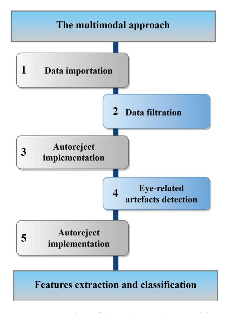
**Figure 2.** An outline of the multimodal approach based on EEG.
The EEG data were given in a CSV file. We used the MNE-Python library to apply advanced preprocessing methods. A "raw" object, a core data structure for continuous EEG data, was created and included information such as channel names and types, standard montage labeling, and the sample rate.
The first step was to filter the EEG signals. This was achieved by applying a digital filter to the data, which suppresses specific frequency components that fall outside of a designated range. There are two main types of digital filters used in digital signal processing (DSP): finite impulse response (FIR) and infinite impulse response (IIR). In the present study, we applied band-pass filtering to the EEG signals using an FIR filter, with a cutoff range of 1–50 Hz. We then segmented the EEG data into one-second non-overlapping epochs. The epochs that had a maximum peak-to-peak signal amplitude of more than 700 μV, or a minimum peak-to-peak signal amplitude of less than 1 μV, were dropped from the dataset, as their existence negatively affected the applicability of the next preprocessing steps. 277
*Sensors* **2023**, *23*, 7350
Afterwards, we employed the Autoreject method to repair or discard corrupted epochs. Bayesian optimization and cross-validation are leveraged in Autoreject to automatically determine an artefact threshold for each channel/sensor; thereafter, faulty channels/sensors are interpolated, or the epoch is discarded. Figure 3 is a diagram depicting the operation of the Autoreject algorithm in a simplified form. For a detailed discussion of how and why this algorithm works, we suggest reading [38], written by the program's creators. To identify and eradicate blinks and other forms of artifactuality, we employed an MNE-Python function that used the EEG channel Fp1 as a surrogate electrooculogram. These components have a lot of variation and tend to be located in the frontotemporal region of the head. The EEG signals were reconstructed after the blinking component was eliminated from the source matrix. Finally, we used Autoreject again to encounter any distortions that could be found after repairing the blink artefacts.
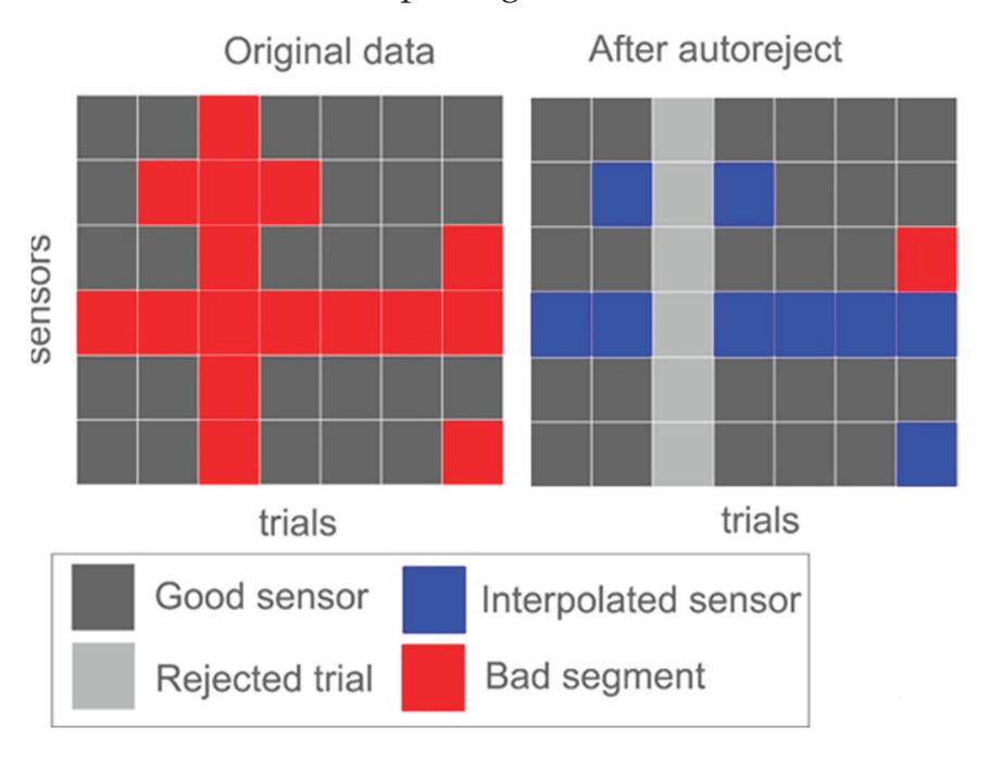
**Figure 3.** A simplified form of the Autoreject algorithm operation.
With more than 80% of the data coming from the NE class, it is possible that the trained model will be biased toward that class. This makes a model's predictions seem naive, even if they have a high degree of accuracy. To counteract the preponderance of the NE class, we undersampled the data with the intention of creating a more even distribution across all classes.
### 3.3. EEG Feature Extraction
After preprocessing the EEG data, two methods that expanded upon previous work on EEG BCI were adopted. First, the EEG data were subjected to specialized spatial filtering in order to boost SNR. We used an algorithm modified from the xDawn algorithm to estimate the spatial filters. Second, we extracted the features from a particular form of the EEG epochs' covariance matrices and adjusted them using techniques from Riemannian geometry. Indeed, the covariance matrices, being Symmetric and Positive-Definite Matrices (SPD), are topologically localized on a Riemannian manifold. To reduce the covariance matrices dimensionality by discarding irrelevant information, we performed the Fisher Geodesic Discriminant Analysis (FGDA) algorithm proposed by [44,45]. Be aware that the features are matrices, rather than the typical vectors. Because we need to maintain the special structure of these matrices, we cannot simply vectorize them. As an alternative, we employed techniques from Riemannian geometry introduced in [46] to map the covariance matrices, belonging to a manifold, onto the Riemannian tangent space, where they may be vectorized and treated as Euclidean objects. Each matrix is represented as a vector of size *n*(*n* + 1)/2, where *n* is the dimension of the SPD matrices. Figure 4 is a geometric depiction of the tangent space mapping process. Despite its more common association with motor imagery, we believe that incorporating it into a visual processing task as part of our research could prove to be useful. A tangent space formed by a group of tangent 278
*Sensors* **2023**, *23*, 7350
vectors can be defined for each point *P*, where *P* ∈ *P*(*n*). Between *P* and the exponential mapping *P* = *Expp*(*Si*), each tangent vector *S* is the derivative at *t* = 0 of the geodesic Γ(*t*), denoted as
$$Exp_{P}(S_{i}) = P^{\frac{1}{2}}exp(P^{-\frac{1}{2}}S_{i}P^{-\frac{1}{2}})P^{\frac{1}{2}}$$
(1)
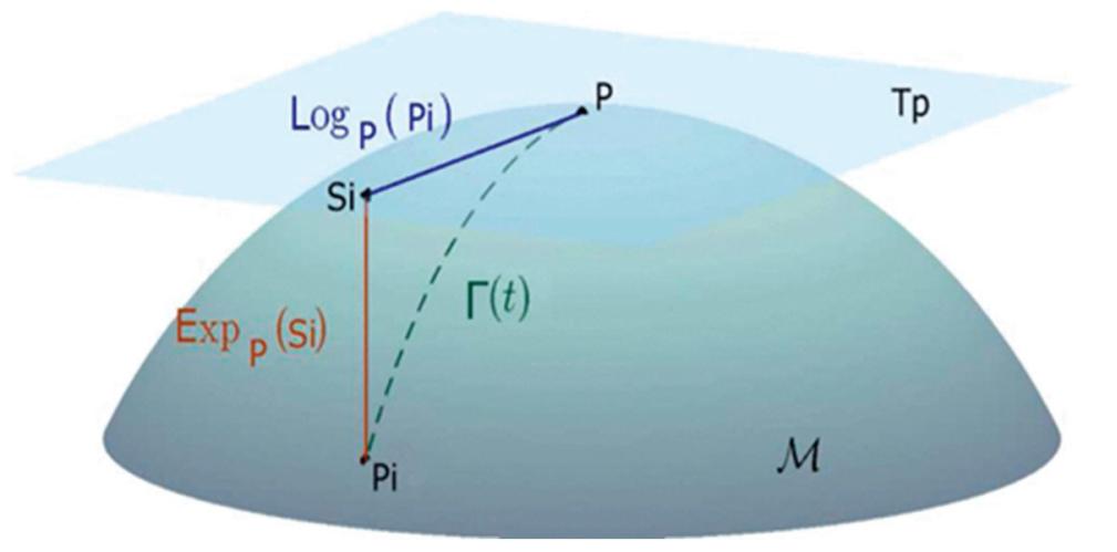
**Figure 4.** A geometric depiction of the tangent space mapping process.
The formula to perform the inverse mapping is denoted as
$$Log_{P}(S_{i}) = P^{\frac{1}{2}}Log_{P}(P^{-\frac{1}{2}}P_{i}P^{-\frac{1}{2}})P^{\frac{1}{2}}$$
$(2)$
Once the tangent space vectors have been extracted, we may use the Principal Component Analysis (PCA) and ANOVA methods as a variable selection strategy to lower the space dimension and alleviate the curse of dimensionality.
### 3.4. EEG Classification
In this study, we rigorously tested multiple ensemble learning algorithms, including Random Forests (RF), Extremely Randomized Trees (ERT), Gradient Tree Boosting (GTB), AdaBoost, and Voting, for their ability to recognize APPD mental states. A modified version of the 5-fold cross-validation process based on stratification was used to assess the quality of the proposed approach.
Five-fold cross-validation is a commonly employed technique in machine learning to assess the performance of algorithms. The method involves dividing the original dataset into five equal-sized subsets, referred to as folds. In turn, each fold serves as the validation data once while the remaining four folds are utilized as training data. This process is repeated five times, with each fold being used exactly once as the validation data. The performance of the algorithm is then evaluated based on the average of the results obtained from the five trials.
This approach to evaluating performance provides a more reliable estimate compared to a single train/test split. This is due to the reduction of variance in performance estimates and the assurance that all data are utilized for both training and testing.
RF: In 2001, L. Breiman presented the Random Forest algorithm as a general-purpose classification and regression technique, and it has since seen tremendous success. The method has been shown to be effective in situations when there are more variables than observations, as it mixes multiple randomized decision trees and averages their predictions. It can be scaled up to address complex issues, customized to meet the needs of a wide range of ad hoc learning projects, and designed to yield metrics of varying significance. The entropy function was used as a metric of split quality in our work, with the number of estimators fixed at 200.
ERT: It is a classifier that works in a way that is similar to RF, but with a slight twist: it introduces randomization to the training process. Each tree in ExtraTrees's multiple trees is 279
*Sensors* **2023**, *23*, 7350
trained independently using the entire dataset used for the classification. The optimum branching at a node is determined by considering a subset of all features, much like the Random Decision Forest. Each feature has a single threshold picked at random rather than multiple, less optimal ones. In our research, we used a total of 200 estimators and the entropy function to evaluate split quality.
GTB: It provides a prediction model in the shape of a collection of weak prediction models, most often decision trees. GTB is the name of the resulting procedure when a decision tree is the weak learner. The method extends the boosting algorithm to any loss function that can be differentiated. In our study, split quality was assessed using the 'friedman\_mse' function and a total of 100 estimators.
AdaBoost: The statistical classification meta-algorithm known as Adaptive Boosting was developed by Yoav Freund and Robert Schapire in 1995. Its performance can be enhanced by combining it with a variety of different learning methods. This method creates a model in which each piece of information is given the same amount of consideration. Incorrectly labelled points are thus given more weight. After this new model is created, the points with greater weights will be given more consideration. A model will be trained repeatedly until a reduced error is received. Because of its rapid convergence to a smaller test error after fewer boosting iterations, the 'SAMME.R' method was chosen in our research.
The hybrid model (Voting): The goal is to predict class labels using a majority vote or the average projected probability (soft vote) based on the results of a collection of machine learning classifiers that are conceptually distinct from one another. A classifier like this can help even out the performance of a group of otherwise comparable models. Based on the outcomes of RF, ERT, and GTB, we used the average projected probability to make predictions about class labels.
### 3.5. Performance Metrics
Several indicators are used to determine the reliability of our findings. The Confusion Matrix is the most important criterion for evaluating our classification models. Metrics like a model's accuracy, precision, and recall are also crucial for understanding how well it actually performs. True positive (TP), false positive (FP), true negative (TN), and false positive (FN) are the four concepts used in the metrics. In greater detail, these metrics are described as follows:
Accuracy: It is the proportion of accurately predicted classes achieved by the model. The formal definition is as follows:
$$Accuracy = �rac{TP + TN}{TP + FP + TN + FN}$$
(3)
Precision: It can be defined as the percentage of positive observations that were successfully anticipated relative to the total number of positive observations that were predicted. The formal definition is as follows:
Precision =
$$\frac{TP}{TP + FP}$$
(4)
Recall: It can be calculated by dividing the number of accurately anticipated positive observations by the total number of observations in the actual class. The formal definition is as follows:
$$Recall = \frac{TP}{TP + FN}$$
(5)
F1-score: It is the weighted average of Precision and Recall. The formal definition is as follows:
F1 – score = 2 ×
$$\frac{Precision \times Recall}{Precision + Recall}$$
(6)
280
*Sensors* **2023**, *23*, 7350
### 4. Results and Discussion
In this study, a multimodal approach was proposed to identify attention-related pilot performance-limiting states based on heterogeneous EEG data. We employed an automated preprocessing pipeline to clean the EEG data by either removing or repairing corrupted epochs. We employed an extraction and selection methodology based on Riemannian geometry analysis to obtain meaningful features from the cleaned data. Using these extracted features, we trained a hybrid ensemble learning model in addition to four other ensemble learning models to detect APPD states.
### 4.1. EEG Signal Analysis
This section presents and discusses the results of employing the automated preprocessing pipeline. Figure 5 reveals the size of the dataset before and after preprocessing the dataset.
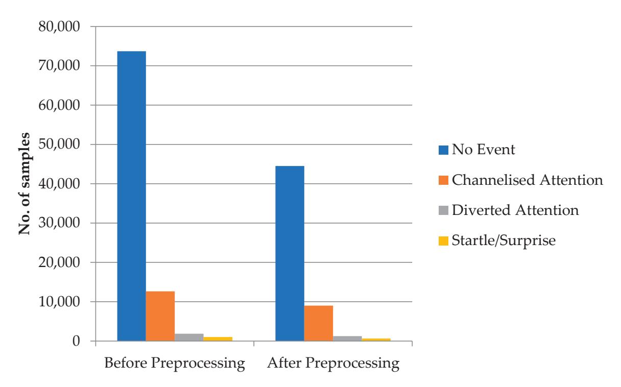
**Figure 5.** The size of the dataset before and after preprocessing the dataset.
We observed that the proposed pipeline identified and discarded a total of 33,786 contaminated epochs in the dataset; to be precise, 29,175 epochs from the NE class, 3632 epochs from the CA class, 598 from the DA class, and 381 epochs from the SS class were dropped from the dataset, as they were considered artefacts.
The proposed EEG preprocessing pipeline aims to improve the quality of EEG data by removing artifacts and other sources of noise, ultimately leading to more accurate and reliable results in downstream analyses. The employed pipeline removed 33,786 out of 89,198 epochs were recorded, resulting in a final dataset of 55,412 epochs. While some may argue that removing such a large number of epochs may lead to a loss of valuable data, it is important to consider the rationale behind the preprocessing steps and the impact they have on the quality of the remaining epochs.
While visually inspecting the discarded epochs, we observed that the epochs were contaminated by physiological artefacts, such as muscle tension and clenching of the jaw, and non-physiological/technical artifacts, such as body movements and powerline interference. As an illustration, Figure 6A depicts an eight-epoch window of the original EEG data, whereas Figure 6B depicts an eight-epoch window of the EEG data that have been preprocessed using the preprocessing pipeline. Figure 6A reveals that ocular activity artefacts, such as blinks and lateral eye movements, were spotted and color-coded as red in epochs 15, 18, and 20. These three epochs were deleted in addition to epochs 19, 21, and 25, as indicated in Figure 6B. We also noticed that some epochs, epoch 16 for instance, were repaired.
281
*Sensors* **2023**, *23*, 7350
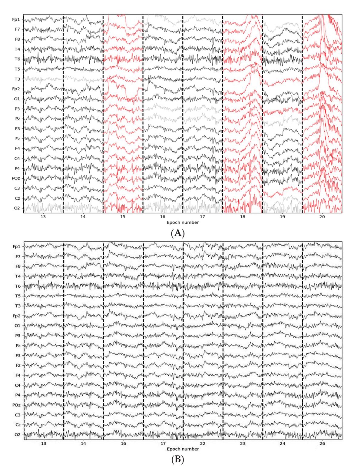
**Figure 6.** An eight-epoch example of the EEG signals before and after preprocessing.
Based on the results presented, the EEG preprocessing pipeline appears to be effective in improving the quality of the EEG data. The visual comparison of the EEG signal before and after preprocessing indicates a reduction in noise and artifacts, resulting in a cleaner and more consistent signal.
The use of Autoreject for artifact rejection and correction, followed by eye-related artefact removal, and a second stage of Autoreject for further correction, provides a comprehensive approach to minimizing the impact of artefacts on the EEG signal. The use of these methods in combination is likely to capture a wide range of artefacts and improve the overall quality of the data.
The effectiveness of the pipeline is also supported by the quantitative analysis of the EEG data. For example, the reduction in the number of epochs removed after preprocessing may indicate that the pipeline was successful in identifying and removing a significant proportion of the artifacts. Furthermore, the comparison of the EEG data before and after preprocessing may provide evidence of the improvements made in the EEG data quality.
However, it is important to note that the effectiveness of the pipeline may depend on various factors, such as the quality of the initial EEG data and the parameters used for each stage of the pipeline. Therefore, a careful evaluation of the resulting EEG data and 282
*Sensors* **2023**, *23*, 7350
the quality of the analysis should be conducted to determine the overall effectiveness of the pipeline.
In addition, while the use of automated methods for artefact detection and correction can provide several advantages, such as consistency and efficiency, they may not capture all sources of noise and artifacts. Therefore, it may be beneficial to supplement the automated methods with visual inspection, especially in cases where subtle sources of noise may be present.
We also report the spectral power analysis of one pilot while performing the highfidelity motion-based flight simulator experiment to examine the overall activity level of the brain at different frequencies. Figure 7 illustrates the spectral power topography during APPD mental states, namely (A) NE, (B) SS, (C) CA, and (D) DA. The power spectral density was computed for each frequency band (delta (0–4 Hz), theta (4–8 Hz), alpha (8–12 Hz), beta (12–30 Hz), and gamma (30–45 Hz)).
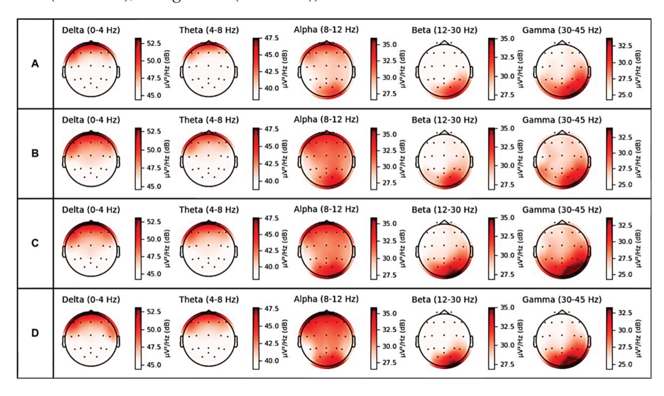
**Figure 7.** Spectral power topography during APPD mental states, namely (**A**) NE, (**B**) SS, (**C**) CA, and (**D**) DA.
In all frequency bands, we commonly found an increase mean power of the CA, DA, and SS states compared to the NE state. We also observed a lower frequency power increase in all frequency band ranges during the SS state. For the delta activity, the highest mean spectral power was located in the frontal lobe during the CA and DA states. For the theta and alpha activity, the highest spectral power was observed in the frontal lobe for theta activity (max: 47.5 dB) and in the frontal and occipital lobes for alpha activity (max: 36.7 dB) during the DA state. Theta oscillations have been linked to mental states of relaxation and drowsiness, while alpha oscillations have been associated with decreased cognitive engagement and mind-wandering. For the beta (max: 33.3 dB) and gamma activity (max: 33 dB), the highest spectral power was observed in the occipital lobe during the CA state. Both beta and gamma oscillations have been connected to engaged cognitive processing, including perception and memory, while beta oscillations have been associated with focused attention and concentration.
Spectral power analysis is a well-established method for analyzing EEG data that has been used in many studies to investigate the spectral properties of the EEG signal. In our study, we used spectral power analysis to visualize the topography of EEG activity during four different mental states—CA, DA, SS, NE. By calculating the power spectral density of the EEG signal in different frequency bands, we were able to obtain topographical maps that showed the distribution of power across the scalp. These maps provided a global view of the EEG patterns that were associated with each mental state, and they allowed us to identify the scalp regions that exhibited the strongest or weakest power in different 283
*Sensors* **2023**, *23*, 7350
frequency bands. This information was useful in identifying patterns of EEG activity that were associated with each mental state, and in validating the results of our subsequent classification analysis. Thus, the use of spectral power analysis was essential to achieving the primary objective of our study, which was to gain a better understanding of the EEG patterns underlying the four mental states.
### 4.2. Evaluation of Machine Learning Models
Five ensemble learning models, namely RF, ERT, GTB, AdaBoost, and Voting, were trained with tangent space features generated from cleaned EEG data using the 5-fold cross-validation technique. First, we estimated the spatial covariance matrices from the cleaned EEG data and obtained a set of SPD matrices of shapes (48, 48). Each matrix was vectorized, obtaining 1176 tangent space features, which were then projected to a lower dimensional space using PCA. In Table 1, we show the performances of the employed ensemble learning models. We considered the macro average of the evaluation metrics Accuracy, Recall, Precision, and F1-score. We also show the standard error, which we calculated based on the F1-score metric for each class because we trained the models using the 5-fold cross-validation technique.
**Table 1.** Ensemble learning models' performances.
| RF | NE | | 91 | 92 | 91 | 0.010 |
|----------|---------------|----|----|----|----|-------|
| | SS | | 82 | 81 | 82 | 0.009 |
| | CA | | 87 | 86 | 87 | 0.013 |
| | DA | | 82 | 83 | 83 | 0.011 |
| | Macro average | 86 | 86 | 86 | 86 | |
| ERT | NE | | 90 | 91 | 90 | 0.011 |
| | SS | | 80 | 80 | 80 | 0.016 |
| | CA | | 86 | 85 | 86 | 0.010 |
| | DA | | 81 | 82 | 82 | 0.012 |
| | Macro average | 84 | 84 | 84 | 84 | |
| GTB | NE | | 91 | 90 | 91 | 0.016 |
| | SS | | 82 | 82 | 82 | 0.009 |
| | CA | | 87 | 87 | 87 | 0.012 |
| | DA | | 83 | 84 | 83 | 0.011 |
| | Macro average | 86 | 86 | 86 | 86 | |
| AdaBoost | NE | | 91 | 88 | 89 | 0.009 |
| | SS | | 80 | 80 | 80 | 0.007 |
| | CA | | 83 | 82 | 83 | 0.010 |
| | DA | | 79 | 81 | 80 | 0.023 |
| | Macro average | 83 | 83 | 83 | 83 | |
| Voting | NE | | 91 | 92 | 92 | 0.013 |
| | SS | | 82 | 82 | 82 | 0.009 |
| | CA | | 87 | 86 | 87 | 0.012 |
| | DA | | 83 | 84 | 83 | 0.013 |
| | Macro average | 86 | 86 | 86 | 86 | |
To provide thorough analysis, the degree of confusion generated by each model was computed. The confusion matrix for the 5-fold cross-validation results using the RF classifier is shown in Figure 8A; the ERT was employed in (B), GTB in (C), AdaBoost in (D), and Voting in (E). The values of the diagonal elements represent the percentage of correctly predicted classes.
284
*Sensors* **2023**, *23*, 7350
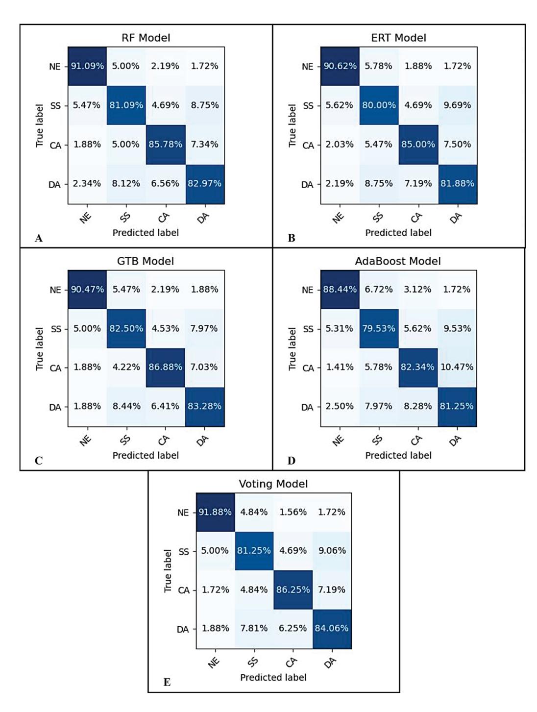
**Figure 8.** The confusion matrix for the 5-fold cross-validation results. The RF model's confusion matrix is shown in (**A**); the ERT in (**B**), GTB in (**C**), AdaBoost in (**D**), and Voting in (**E**).
Based on the data from Table 1, we observed that all five models provided good detection performances. The best accuracy performance achieved was 86%, which was achieved by the RF, GTB, and Voting models, followed by AdaBoost (84%) and ERT (83%). The same trend can be seen across different metrics, including precision, recall, and F1-score. We believe the reason why ERT did not perform as well as the RF model, although both algorithms are based on the bagging or bootstrap aggregation technique, is because of the randomness in the way splits are computed; while the most discriminative thresholds are picked as the splitting rule in RF, thresholds in ERT are drawn at random, which slightly increased biasness in the model. Similarly, we also observed a slight difference in the performances of GTB and AdaBoost, even though both algorithms are based on the boosting technique. We suspect the reason of the increase in GTB model performance is due to the use of the log loss function, which is more robust to mislabeled examples in the dataset; unlike GTB, the AdaBoost algorithm uses the exponential loss function.
Figure 8 further shows that all models made accurate classification predictions. The NE mental state was predicted by all five models to be the easiest to distinguish, with an accuracy performance range of 88.44–91.88%, followed by the CA with a range of 82.34–86.88%. It was also discovered that, across all five models, DA was the third best at recognizing class with an accuracy performance of 81.25–84.06%, while SS was the worst at recognizing class with an accuracy performance of 79.53–82.50%. Nevertheless, 285
*Sensors* **2023**, *23*, 7350
these performance levels can be enhanced if the dataset is more cohesive. With regards to predicting NE and DA states, the Voting classifier performed best, whereas the GTB classifier performed best with regards to predicting CA and SS states.
The use of ensemble models has become increasingly popular in machine learning due to their ability to leverage the strengths of different models to improve performance. In this study, we compared the performance of several popular ensemble models, including RF, ERT, GTB, and AdaBoost, with a hybrid ensemble model. The results showed that the hybrid ensemble model outperformed ERT and AdaBoost and achieved comparable performance to RF and GTB. One of the key advantages of the hybrid ensemble model is its flexibility. By combining different models, the hybrid ensemble approach can handle various types of data and tasks, making it a versatile option for different applications. In contrast, the other models tested in this study were each based on a single algorithm, limiting their flexibility to some extent. Another advantage is its improved generalization ability. The use of a combination of models in the hybrid ensemble approach can help to mitigate the risk of overfitting. This can lead to more accurate predictions on new, unseen data, making the hybrid ensemble model a promising approach for practical applications.
Several studies have investigated the classification of mental states using EEG data. However, some of these studies did not make their dataset publicly accessible, did not achieve clear or consistent results, employed different sensors and conventional preprocessing techniques, or did not classify the same number of mental states. In order to compare the results of our multimodal approach with other studies, we evaluated our approach in the context of studies that have used the same dataset.
Harrivel et al. [35] implemented a broad suite of sensors to classify pilot mental states. Although this study provided initial insights into the use of physiological signals to measure attention in aviation, their datasets were limited in size. In addition, their results were not conclusive because they were based on only one pilot. Harrivel et al. [34], on the other hand, considered a larger sample size and employed multiple sensors, including EEG, ECG, GSR, and respiration. However, the study relied on spectral power features and did not classify four mental states. Moreover, the results were not as good as in our study, likely due to the limited classification capabilities of spectral power features. Similarly, [20] considered a larger sample size of 18 users but did not clean their data from artifacts and merged three mental states into one called the event state. The lack of artifact removal may have contributed to unclear results, and the use of different metrics limited comparison with our study.
We also evaluated our approach in the context of studies that have used a different dataset. For example, Han et al. [25], proposed a multimodal deep learning network to classify four mental states (distraction, baseline, workload, and fatigue) using a dataset of eight pilots. The authors employed conventional preprocessing techniques, including filtering and ICA for removing eye-related artifacts. They also extracted PSD features from the EEG signals and provided three topographic maps as inputs to a CNN model. In addition, the authors employed ECG, GSR, and respiration signals as inputs to an LSTM network. However, the dataset used by Han et al. was not a publicly accessible dataset, unlike our study and studies [20,29,34,35], which were all publicly available. While their results were promising, the small sample size and lack of a public dataset may limit the generalizability of the findings. In addition, our approach achieved an accuracy of 86% in detecting mental states, which is a substantial improvement over Han et al. study's performance of 77.7%. Hernández-Sabaté et al. [43] developed a CNN model to classify different mental workloads of pilots using EEG signals. Although they made their dataset publicly available, they divided a signal state to multiple states.
In comparison to our previous study [29], where we evaluated the impact of different preprocessing techniques on the performance of ML algorithms for classifying pilots' mental states, the current study represents a significant improvement in mental state detection.
In this study, we developed a novel multimodal approach that includes advanced automated preprocessing techniques, Riemannian geometry-based feature extraction, and 286
*Sensors* **2023**, *23*, 7350
a hybrid ensemble learning technique that combines the results of several machine learning classifiers. The use of Riemannian geometry analysis for feature extraction and the hybrid ensemble learning technique outperforms traditional approaches and shows the importance of advanced techniques in improving the accuracy of mental state detection. Our approach is the first of its kind because it combines advanced techniques proposed in three different fields: Autoreject, from the neuroscience field for data preprocessing; Tangent space mapping, from BCI for feature extraction; and hybrid ensemble learning artificial intelligence for pilot's mental states classification.
This study can have significant implications for improving pilots' performance and safety in the aviation industry. Our approach has the potential to benefit several sectors within the aviation industry. One important application is in pilot training and performance evaluation. By accurately characterizing pilot mental states using EEG data, the proposed approach can be used to identify areas where pilots may need additional training or support, and to evaluate the effectiveness of training programs in improving cognitive performance.
Another potential application is in aviation safety, particularly in identifying potential safety hazards related to pilot mental states. By providing a detailed and accurate characterization of pilot mental states during flight, the proposed approach can help identify situations where pilots may be at higher risk of making errors or experiencing cognitive overload, allowing for proactive interventions to be taken to prevent accidents and improve safety.
Additionally, our approach has the potential to improve human–machine interaction in the aviation industry. By using EEG data to monitor pilot mental states, future BCI systems can be developed that are better able to adapt to the cognitive state of the pilot, improving the efficiency and safety of the aviation system as a whole.
Overall, the potential applications of our approach are diverse and have the potential to make a significant contribution to the aviation industry by improving safety, training, and human–machine interaction.
#### 5. Conclusions
We conducted an exploratory investigation using uncontaminated EEG data and ensemble learning algorithms to characterize the pilot's mental states (i.e., channelized attention, diverted attention, startle/surprise, and normal). We also demonstrated how the pilot's varied mental states impacted physiological indicators. With the goal of identifying the neural signal related to cognitive processes reflective of brain activity while disregarding the other artefacts and extracting significant information, we proposed a feasible approach for automatically preprocessing EEG data. In order to proceed to the classification phase, the processed data underwent feature extraction, during which spatial covariance matrices were calculated and subsequently mapped onto the Riemannian tangent space. Four ensemble learning models, namely RF, ERT, GTB, and AdaBoost, and a hybrid ensemble model were trained using tangent space vectors.
Based on the findings, it was clear that the proposed method successfully identified artifacts in the EEG epochs and either fixed or discarded them automatically. In addition, the results indicated the viability of implementing EEG-based BCI systems, such as tangent space mapping, to characterize the pilot's mental states. According to the findings of the pilot's mental states detection investigation, we observe that the RF, GTB, and the hybrid ensemble models are the best at predicting NE, CA, SS, and DA states, with an accuracy rate of 86%.
The innovative nature of this study lies in its combination of advanced automated preprocessing techniques, Riemannian geometry-based feature extraction, and ensemble learning models, which, together, provide a detailed and accurate characterization of pilot mental states, ultimately leading to a safer and more efficient aviation system.
The models' performances will be further refined, and the training dataset will be enlarged, in subsequent work. We also aim to apply the aforementioned approach to a 287
*Sensors* **2023**, *23*, 7350
broad range of machine learning and deep learning models. In further studies, we can also investigate the possibility of extracting other meaningful features.
**Author Contributions:** Conceptualization, I.A. and I.M.; methodology, I.A. and I.M.; software, I.A.; validation, I.A. and I.M.; formal analysis, I.A.; investigation, I.A.; data curation, I.A.; writing—original draft preparation, I.A.; writing—review and editing, I.M. and K.W.J.; visualization, I.A.; supervision, I.M. and K.W.J. All authors have read and agreed to the published version of the manuscript.
**Funding:** The APC was funded by Cranfield University.
**Institutional Review Board Statement:** Not applicable.
**Informed Consent Statement:** Not applicable.
**Data Availability Statement:** The source code and the data used for the experiments are made freely available under the MIT License and can be downloaded from https://doi.org/10.17862/cranfield. rd.22232062 (accessed on 1 July 2023).
**Conflicts of Interest:** The authors declare no conflict of interest.
#### Appendix A
*Appendix A.1. Advanced Brain Monitoring X24 EEG Headset*
The X24 EEG headset was employed to gather the EEG dataset. This headset offers a wireless option for acquiring and recording EEG signals without the need for scalp abrasion. It is equipped with 20 electrodes arranged in the standard 10–20 format and one additional electrode, POz, as shown in Figure A1. These electrodes are located at specific locations on the head, such as Fz, Cz, Pz, F3, F4, C3, C4, P3, P4, O1, O2, T5, T3, F7, Fp1, Fp2, F8, T4, T6, and Linked Mastoids. The wireless technology allows for freedom of movement for the user during data collection and display in real-time. The headset collects EEG signals from the sensors on the participant and processes the signals through analog-to-digital conversion, encoding, formatting, and transmission. It operates at a sample rate of 256 Hz and uses the system's bi-directional capabilities to check scalp-electrode impedance and monitor battery capacity in the X24 Headset. Figure A1 illustrates the names and locations of the electrodes on the EEG sensor.
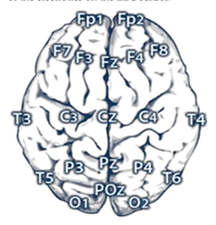
**Figure A1.** EEG electrode names and locations.
*Appendix A.2. Flight Simulator*
The dataset was obtained from 18 commercial aviation pilots who participated in a research flight deck simulation at NASA Langley Research Center. The flight deck, which is known as the cockpit motion facility, is an all-glass reconfigurable cockpit that
288
*Sensors* **2023**, *23*, 7350
is equipped with a programmable sidestick and pedal control inceptors. The simulator, which can operate in both motion-based and fixed-base modes, is designed to provide a high-fidelity, full-systems flight experience for pilots. It is used to evaluate and improve research concepts related to flight crew operations, covering everything from engine startup to engine shutdown.
#### References
- 1. Kelly, D.; Efthymiou, M. An Analysis of Human Factors in Fifty Controlled Flight into Terrain Aviation Accidents from 2007 to 2017. *J. Saf. Res.* **2019**, *69*, 155–165. [CrossRef] [PubMed]
- 2. Yen, J.R.; Hsu, C.C.; Yang, H.; Ho, H. An Investigation of Fatigue Issues on Different Flight Operations. *J. Air Transp. Manag.* **2009**, *15*, 236–240. [CrossRef]
- 3. Hankins, T.C.; Wilson, G.F. A Comparison of Heart Rate, Eye Activity, EEG and Subjective Measures of Pilot Mental Workload during Flight. *Aviat. Space Environ. Med.* **1998**, *69*, 360–367. [PubMed]
- 4. Boksem, M.A.S.; Tops, M. Mental Fatigue: Costs and Benefits. *Brain Res. Rev.* **2008**, *59*, 125–139. [CrossRef]
- 5. International Air Transport Association. *2021 Safety Report Edition*; International Air Transport Association: Montreal, QC, Canada, 2022.
- 6. International Air Transport Association. *Loss of Control In-Flight Accident Analysis Report 2019 Edition*; International Air Transport Association: Montreal, QC, Canada, 2019; ISBN 9789292640026.
- 7. Commercial Aviation Safety Team SE211: Airplane State Awareness—Training for Attention Management. Available online: http://www.skybrary.aero/index.php/SE211:\_Airplane\_State\_Awareness\_-\_Training\_for\_Attention\_Management\_(R-D) (accessed on 25 December 2022).
- 8. Hogervorst, M.A.; Brouwer, A.M.; van Erp, J.B.F. Combining and Comparing EEG, Peripheral Physiology and Eye-Related Measures for the Assessment of Mental Workload. *Front. Neurosci.* **2014**, *8*, 322. [CrossRef]
- 9. Liu, Y.; Ayaz, H.; Shewokis, P.A. Multisubject "Learning" for Mental Workload Classification Using Concurrent EEG, FNIRS, and Physiological Measures. *Front. Hum. Neurosci.* **2017**, *11*, 389. [CrossRef]
- 10. Bigdely-Shamlo, N.; Mullen, T.; Kothe, C.; Su, K.M.; Robbins, K.A. The PREP Pipeline: Standardized Preprocessing for Large-Scale EEG Analysis. *Front. Neuroinform.* **2015**, *9*, 16. [CrossRef]
- 11. Fló, A.; Gennari, G.; Benjamin, L.; Dehaene-Lambertz, G. Automated Pipeline for Infants Continuous EEG (APICE): A Flexible Pipeline for Developmental Cognitive Studies. *Dev. Cogn. Neurosci.* **2022**, *54*, 101077. [CrossRef]
- 12. Kordylewski, H.; Graupe, D.; Liu, K. A Novel Large-Memory Neural Network as an Aid in Medical Diagnosis Applications. *IEEE Trans. Inf. Technol. Biomed.* **2001**, *5*, 202–209. [CrossRef]
- 13. Güler, I.; Übeyli, E.D. Adaptive Neuro-Fuzzy Inference System for Classification of EEG Signals Using Wavelet Coefficients. *J. Neurosci. Methods* **2005**, *148*, 113–121. [CrossRef]
- 14. Übeyli, E.D. Wavelet/Mixture of Experts Network Structure for EEG Signals Classification. *Expert. Syst. Appl.* **2008**, *34*, 1954–1962. [CrossRef]
- 15. Stancin, I.; Cifrek, M.; Jovic, A. A Review of EEG Signal Features and Their Application in Driver Drowsiness Detection Systems. *Sensors* **2021**, *21*, 3786. [CrossRef] [PubMed]
- 16. Roza, V.C.C.; Postolache, O.A. Multimodal Approach for Emotion Recognition Based on Simulated Flight Experiments. *Sensors* **2019**, *19*, 5516. [CrossRef] [PubMed]
- 17. Jiang, X.; Bian, G.B.; Tian, Z. Removal of Artifacts from EEG Signals: A Review. *Sensors* **2019**, *19*, 987. [CrossRef] [PubMed]
- 18. Ziegler, M.D.; Kraft, A.; Krein, M.; Lo, L.C.; Hatfield, B.; Casebeer, W.; Russell, B. Sensing and Assessing Cognitive Workload across Multiple Tasks. In *Foundations of Augmented Cognition: Neuroergonomics and Operational Neuroscience*; Lecture Notes in Computer Science (Including Subseries Lecture Notes in Artificial Intelligence and Lecture Notes in Bioinformatics); Springer: Cham, Switzerland, 2016; Volume 9743, pp. 440–450.
- 19. Jiao, Z.; Gao, X.; Wang, Y.; Li, J.; Xu, H. Deep Convolutional Neural Networks for Mental Load Classification Based on EEG Data. *Pattern Recognit.* **2018**, *76*, 582–595. [CrossRef]
- 20. Terwilliger, P.; Sarle, J.; Walker, S.; Terwilliger, P.; Sarle, J.; Walker, S. A ResNet Autoencoder Approach for Time Series Classification of Cognitive State A ResNet Autoencoder Approach for Time Series Classification of Cognitive State. *MODSIM World* **2020**, 1–11.
- 21. Jaquess, K.J.; Gentili, R.J.; Lo, L.C.; Oh, H.; Zhang, J.; Rietschel, J.C.; Miller, M.W.; Tan, Y.Y.; Hatfield, B.D. Empirical Evidence for the Relationship between Cognitive Workload and Attentional Reserve. *Int. J. Psychophysiol.* **2017**, *121*, 46–55. [CrossRef]
- 22. Nittala, S.K.R.; Elkin, C.P.; Kiker, J.M.; Meyer, R.; Curro, J.; Reiter, A.K.; Xu, K.S.; Devabhaktuni, V.K. Pilot Skill Level and Workload Prediction for Sliding-Scale Autonomy. In Proceedings of the 17th IEEE International Conference on Machine Learning and Applications, ICMLA 2018, Orlando, FL, USA, 17–20 December 2019; pp. 1166–1173. [CrossRef]
- 23. Johnson, M.K.; Blanco, J.A.; Gentili, R.J.; Jaquess, K.J.; Oh, H.; Hatfield, B.D. Probe-Independent EEG Assessment of Mental Workload in Pilots. In Proceedings of the International IEEE/EMBS Conference on Neural Engineering, NER, Montpellier, France, 22–24 April 2015; Volume 2015, pp. 581–584.
- 24. Zhang, P.; Wang, X.; Chen, J.; You, W. Feature Weight Driven Interactive Mutual Information Modeling for Heterogeneous Bio-Signal Fusion to Estimate Mental Workload. *Sensors* **2017**, *17*, 2315. [CrossRef]
- 25. Han, S.Y.; Kwak, N.S.; Oh, T.; Lee, S.W. Classification of Pilots' Mental States Using a Multimodal Deep Learning Network. *Biocybern. Biomed. Eng.* **2020**, *40*, 324–336. [CrossRef]
289
*Sensors* **2023**, *23*, 7350
- 26. Binias, B.; Myszor, D.; Cyran, K.A. A Machine Learning Approach to the Detection of Pilot's Reaction to Unexpected Events Based on EEG Signals. *Comput. Intell. Neurosci.* **2018**, *2018*, 2703513. [CrossRef]
- 27. Oh, H.; Hatfield, B.D.; Jaquess, K.J.; Lo, L.C.; Tan, Y.Y.; Prevost, M.C.; Mohler, J.M.; Postlethwaite, H.; Rietschel, J.C.; Miller, M.W.; et al. A Composite Cognitive Workload Assessment System in Pilots under Various Task Demands Using Ensemble Learning. In *Foundations of Augmented Cognition: Neuroergonomics and Operational Neuroscience*; Lecture Notes in Computer Science (Including Subseries Lecture Notes in Artificial Intelligence and Lecture Notes in Bioinformatics); Springer: Cham, Switzerland, 2015; Volume 9183, pp. 91–100.
- 28. Wu, E.Q.; Peng, X.Y.; Zhang, C.Z.; Lin, J.X.; Sheng, R.S.F. Pilots' Fatigue Status Recognition Using Deep Contractive Autoencoder Network. *IEEE Trans. Instrum. Meas.* **2019**, *68*, 3907–3919. [CrossRef]
- 29. Alreshidi, I.M.; Moulitsas, I.; Jenkins, K.W. *Miscellaneous EEG Preprocessing and Machine Learning for Pilots' Mental States Classification: Implications*; Association for Computing Machinery: New York, NY, USA, 2022; ISBN 9781450396943.
- 30. Jas, M.; Engemann, D.A.; Bekhti, Y.; Raimondo, F.; Gramfort, A. Autoreject: Automated Artifact Rejection for MEG and EEG Data. *Neuroimage* **2017**, *159*, 417–429. [CrossRef] [PubMed]
- 31. Bonassi, A.; Ghilardi, T.; Gabrieli, G.; Truzzi, A.; Doi, H.; Borelli, J.L.; Lepri, B.; Shinohara, K.; Esposito, G. The Recognition of Cross-Cultural Emotional Faces Is Affected by Intensity and Ethnicity in a Japanese Sample. *Behav. Sci.* **2021**, *11*, 59. [CrossRef]
- 32. Pousson, J.E.; Voicikas, A.; Bernhofs, V.; Pipinis, E.; Burmistrova, L.; Lin, Y.P.; Griškova-Bulanova, I. Spectral Characteristics of Eeg during Active Emotional Musical Performance. *Sensors* **2021**, *21*, 7466. [CrossRef]
- 33. Wang, X.W.; Nie, D.; Lu, B.L. Emotional State Classification from EEG Data Using Machine Learning Approach. *Neurocomputing* **2014**, *129*, 94–106. [CrossRef]
- 34. Harrivel, A.R.; Stephens, C.L.; Milletich, R.J.; Heinich, C.M.; Last, M.C.; Napoli, N.J.; Abraham, N.A.; Prinzel, L.J.; Motter, M.A.; Pope, A.T. Prediction of Cognitive States during Flight Simulation Using Multimodal Psychophysiological Sensing. In Proceedings of the AIAA Information Systems—AIAA Infotech at Aerospace, Grapevine, TX, USA, 9–13 January 2017; American Institute of Aeronautics and Astronautics: Reston, VA, USA, 2017.
- 35. Harrivel, A.R.; Liles, C.A.; Stephens, C.L.; Ellis, K.K.; Prinzel, L.J.; Pope, A.T. Psychophysiological Sensing and State Classification for Attention Management in Commercial Aviation. In Proceedings of the AIAA Infotech @ Aerospace Conference, San Diego, CA, USA, 4–8 January 2016; American Institute of Aeronautics and Astronautics Inc., AIAA: Crew Systems and Aviation Operations Branch, NASA Langley Research Center: Hampton, VA, USA, 2016.
- 36. Barachant, A.; Bonnet, S.; Congedo, M.; Jutten, C. Multiclass Brain-Computer Interface Classification by Riemannian Geometry. *IEEE Trans. Biomed. Eng.* **2012**, *59*, 920–928. [CrossRef]
- 37. Majidov, I.; Whangbo, T. Efficient Classification of Motor Imagery Electroencephalography Signals Using Deep Learning Methods. *Sensors* **2019**, *19*, 1736. [CrossRef]
- 38. Singh, A.; Lal, S.; Guesgen, H.W. Reduce Calibration Time in Motor Imagery Using Spatially Regularized Symmetric Positives-Definite Matrices Based Classification. *Sensors* **2019**, *19*, 379. [CrossRef]
- 39. Appriou, A.; Pillette, L.; Trocellier, D.; Dutartre, D.; Cichocki, A.; Lotte, F. BioPyC, an Open-Source Python Toolbox for Offline Electroencephalographic and Physiological Signals Classification. *Sensors* **2021**, *21*, 5740. [CrossRef]
- 40. Dehais, F.; Duprès, A.; Blum, S.; Drougard, N.; Scannella, S.; Roy, R.N.; Lotte, F. Monitoring Pilot's Mental Workload Using Erps and Spectral Power with a Six-Dry-Electrode EEG System in Real Flight Conditions. *Sensors* **2019**, *19*, 1324. [CrossRef]
- 41. Avots, E.; Jermakovs, K.; Bachmann, M.; Päeske, L.; Ozcinar, C.; Anbarjafari, G. Ensemble Approach for Detection of Depression Using EEG Features. *Entropy* **2022**, *24*, 211. [CrossRef]
- 42. Zhang, P.; Wang, X.; Zhang, W.; Chen, J. Learning Spatial-Spectral-Temporal EEG Features with Recurrent 3D Convolutional Neural Networks for Cross-Task Mental Workload Assessment. *IEEE Trans. Neural Syst. Rehabil. Eng.* **2019**, *27*, 31–42. [CrossRef] [PubMed]
- 43. Hernández-Sabaté, A.; Yauri, J.; Folch, P.; Piera, M.À.; Gil, D. Recognition of the Mental Workloads of Pilots in the Cockpit Using EEG Signals. *Appl. Sci.* **2022**, *12*, 2298. [CrossRef]
- 44. Barachant, A.; Bonnet, S.; Congedo, M.; Jutten, C. Riemannian Geometry Applied to BCI Classification. In Proceedings of the LVA/ICA 2010—9th International Conference on Latent Variable Analysis and Signal Separation, St. Malo, France, 27–30 September 2010.
- 45. Barachant, A.; Bonnet, S.; Congedo, M.; Jutten, C. Classification of Covariance Matrices Using a Riemannian-Based Kernel for BCI Applications. *Neurocomputing* **2013**, *112*, 172–178. [CrossRef]
- 46. Barachant, A. *MEG Decoding Using Riemannian Geometry and Unsupervised Classification*; Grenoble University: Grenoble, France, 2014; pp. 1–8.
**Disclaimer/Publisher's Note:** The statements, opinions and data contained in all publications are solely those of the individual author(s) and contributor(s) and not of MDPI and/or the editor(s). MDPI and/or the editor(s) disclaim responsibility for any injury to people or property resulting from any ideas, methods, instructions or products referred to in the content.
290
MDPI St. Alban-Anlage 66 4052 Basel Switzerland www.mdpi.com
*Sensors* Editorial Office E-mail: sensors@mdpi.com www.mdpi.com/journal/sensors

Disclaimer/Publisher's Note: The statements, opinions and data contained in all publications are solely those of the individual author(s) and contributor(s) and not of MDPI and/or the editor(s). MDPI and/or the editor(s) disclaim responsibility for any injury to people or property resulting from any ideas, methods, instructions or products referred to in the content.

Academic Open Access Publishing
mdpi.com ISBN 978-3-7258-0082-7